
qEEG Normative Databases
ORIENTATION AND OUTLINE
This unit reviews basic concepts related to qEEG databases, including purposes, development methods, history, and a description of several currently used databases.
It is important that the clinician evaluates the claims made by product developers to determine if the claimed methods and product features are valid. This may present some difficulty for clinicians not experts in database development, statistical analysis, EEG theory, and practice.
Some databases discussed here were developed using client EEGs rather than carefully screened subjects. The claim that such individuals’ EEG recordings can be “cleaned” of abnormal patterns to allow their data to be included in a normative database is questionable at best. Additionally, using recordings from clinical subjects, the clinical database approach depends upon the developer’s knowledge and understanding of neurophysiology, neuropsychology, electroencephalography, and more. Therefore, some of these may be effective, valid, and useful in clinical settings, while others may not.
Ultimately the clinician is responsible for using a reliable, validated instrument with known and well-documented parameters that have withstood the scrutiny of multiple peer-reviewed publications. One or two publications the developer(s) authored do not meet these criteria.
International QEEG Certification Board Blueprint Coverage
This unit covers IX. A. Knowledge regarding limits of interpreting QEEG regarding choice of reference databases and recognizing statistical probability versus clinical probability.

This unit reviews Introduction and Definitions, Purposes of qEEG Normative Databases, Contents of qEEG Normative Databases, Probability and Statistics Basics for Database Use, Ethics Review with Institutional Review Board, Subjects, Data for qEEG Normative Databases, Reliability and Validity, History, Features of Selected Current Databases, and Summary.
INTRODUCTION AND DEFINITIONS
In its broadest sense, a database is a repository of information about something of interest organized and kept in a manner that can easily be accessed for a particular purpose. The storage repository or method is digitized and electronic, enabling quick data access. Especially for qEEG normative databases, clinicians often use the data to generate diagrams or maps that depict how brain function is distributed and for neurofeedback.
Despite the value of digitization, visual inspection of the analog waveforms of the EEG remains especially important. Not only does visual inspection often serve as the basis for creating a template for artifacting, but it can provide a qualitative description of a subject’s record, which is also amenable to some degree of quantification. However, the EEG can also be analyzed mathematically and with greater reliability than visual inspection for many EEG variables. The quantitative EEG (qEEG) rapidly produces quantified values for many variables.
Depending on the content of interest and variables involved, organizing a database may be more or less elaborate. Variables from EEG analysis, such as frequency band and coherence, age range, and recording condition, are typically used to organize the data that comprise a qEEG normative database.
Variables and Values
A variable is any characteristic that can be observed or counted. For instance, EEG variable characteristics include power in the alpha band or coherence between Fp1 and Fp2 for the beta band.Variables can take on or vary between any of a number of values. For example, the variable of EEG alpha power can take on values ranging from zero to many microvolts, or theta coherence between two 10-20 sites may vary between different amounts of coherence (cf. Australian Bureau of Statistics, 2023). EEG variables in a qEEG database may be relevant for clinical or experimental purposes.
Structure and Scales of Measurement
The qEEG is organized using qualitative data (Anastasi, 1976; University of New South Wales, 2023). Qualitative categories (e.g., nominal and ordinal scales) define the conditions under which the data were collected.A nominal scale is used for discrete categories of information. For example, the data may have been collected when the subject rested with her eyes open or closed or when performing an auditory or visual attention task.
An ordinal scale is used for age ranges and frequency bands that follow one another in sequence, or order, with the size of the age range or frequency band not necessarily equal from one step to the next.
A qEEG database, therefore, has more than one dimension (e.g., the data collection condition, age range, EEG variables) that together form a virtual matrix of cells in which qEEG data are stored. EEG variables' means and standard deviations are key elements in the database’s organizational matrix.
Although qEEG databases organize their data by qualitative category, databases have quantitative data in each given category or intersection of categories. This results in a cell of the matrix described above (e.g., resting eyes closed, 8-10 Hz alpha power for 20–30-year-olds). Although quantitative data can sometimes be discrete and take on only whole numbers (e.g., number of children), qEEG databases use 20–30-year-olds that can take on values measured or broken down to several decimal places of accuracy.
The data in qEEG databases are also at a ratio scale where an absolute value of zero can occur and where the “distance” between 1 and 2 is the same as between 10 and 11.
By contrast, an interval scale is also continuous. It has an equal “distance” between adjacent values (e.g., 1 and 2 and 10 and 11). Still, it does not have a true zero or complete absence of whatever is being measured (e.g., degrees Fahrenheit or Celsius have no absolute zero). Like other modern databases, qEEG databases are digital and saved for quick computer-based access and use.
Norms
A norm may be qualitative or categorical, or quantified in nature. A qEEG norm for the variable of alpha band amplitude, measured at a posterior 10-20 site in a healthy adult with eyes closed, is in the range of 20-60 uV (Lewine & Orrison, 1995). qEEG normative databases, however, quantify the expected range of values such variables can assume. They quantify variables with specific average or mean values and measure of variability or standard deviation for the variable’s range. qEEG norms, then, quantify what is normal for the subjects selected to meet expectations for normal health and whose EEG data were then collected, as will be described further below.
qEEG norms are electronic tables, consisting of means and standard deviations for calculated EEG variables. For example, for each 10-20 site and pairs of sites where the EEG has been collected from normal healthy individuals in adjacent age groups, from various states and tasks. The quantified EEG data are organized by qualitative variables (i.e., 10-20 site, site pairs, age group, state or type of task) because the normal EEG is affected by those variables. qEEG norms reveal deviations from normalcy. They may suggest impairments, which may be confirmed by other diagnostic information (e.g., neurological examination or neuropsychological testing), and possibly by treatment (e.g., neurofeedback training).
Purposes of qEEG Normative Databases
Developers of databases begin by formulating a purpose for the database.Description
qEEG database norms serve several purposes. Generally, qEEG norms characterize or describe the range of what is expected for particular EEG variables seen in healthy subjects. In this, they are similar to norms used in healthcare for height and weight. As Anastasi writes regarding psychological test scores, “Norms represent the test performance of the standardization sample. The norms are thus empirically established by determining what a representative group of persons do on a test. Any individual’s raw score is then referred to the distribution of scores obtained by the standardization sample to discover where he falls in that distribution (Anastasi, 1976, p. 67).” The norms of the qEEG database have a descriptive purpose that presents what is normal for the sample of healthy individuals selected to represent the entire population of healthy people.
Comparison
A normative description of the mean and variability of alpha power in a group of healthy subjects in a resting eyes-closed condition, can also serve the purpose of a benchmark. We can use it to compare a new client to normal values. Is the client’s EEG consistent with normal expectations or does it deviate from them?
A database user may ask, “Does this client’s alpha power conform with the prediction I would make based on the normal range of alpha power?” This comparative purpose resembles the medical practice of evaluating a patient’s blood pressure in relation to the normal expectation for the range of blood pressure values for healthy people of similar age to the patient.
The comparative purpose of norms addresses what Anastasi (1976) writes in the context of psychological test theory about test scores, which applies equally to the value of an EEG variable of any individual subject: “In the absence of additional interpretive data, a raw score on any psychological test is meaningless (p. 67).”
To give meaning to a subject’s EEG finding, one must place it in context. The basic statistical methods described below are used to quantify the degree of difference from expectation and its statistical significance.
Diagnosis
In clinical settings, findings that a client’s EEG differs from the norm may be integrated with other assessment findings to understand better and diagnose problems presented by the client. However, deviations from the norms in a qEEG database are not diagnostic.
A statistically significant difference between client EEG findings and norms in a qEEG database may not be clinically significant. It may not predict how a client functions in their daily activities. Deviations from database norms can suggest hypotheses to explore. Together with information from other sources, they may contribute to making a valid diagnosis by a qualified health provider.
Clinicians should consider qEEG findings in the context of clinical presentation, medical history, findings of other relevant tests, and understanding of the anatomy, physiology, and function of the brain together with a knowledge of base rates in the setting where the clinician works (i.e., the frequencies of diagnoses). These factors highlight the limitations of qEEG findings.
Biomarkers
Biomarkers are biological markers, being “objective indications of medical state observed from outside the patient – which can be measured accurately and reproducibly” (Strimbu & Tavel, 2010, p. 463). Related to biomarkers are endophenotypes (i.e., “within phenotypes”), quantifiable phenomena that link underlying biological processes to symptoms and are more stable than the symptoms.
McVoy, Lytle, Fulchiero, Aebi, Adeleye, and Sajatovic (2019), for example, present a recent review of possible biomarkers in child psychiatric disorders. Several databases have been used to explore EEG biomarkers and endophenotypes, examples of which are for ADHD (Arns, Gunkelman, Breteler, & Spronk, 2008; Ji, Choi, Lee, Yoon, Won, Jeong, Kang, & Kim, 2022), Alzheimer’s disease (Jeong, Park, & Kang, 2022), Parkinson’s disease (Caviness, Utianski, Hentz, Beach, Dugger, Shill, Driver-Dunckley, Sabbagh, Mehta, & Adler, 2016 and traumatic brain injury (Thatcher, Walker, Gerson, & Geisler, 1989).
Development of Training Protocols
qEEG database norms can also be compared in neurofeedback training. Significant differences between a client’s EEG and the qEEG normative database may be used in planning a neurofeedback training course. In neurofeedback training, a client’s instantaneous EEG can be compared to normative values to provide the basis for delivering feedback, for example, in z-score neurofeedback.
Evaluation of Training
Differences between the client’s EEG and normative values, seen before and after neurofeedback or some other intervention, can also be compared to determine whether the client’s EEG has normalized, to evaluate treatment outcomes.
Scientific Discovery
In a research setting, a special group (e.g., individuals with major depression or mild traumatic brain injury) may be compared to the normative group in the qEEG database to identify what best differentiates the two groups. For example, investigators can utilize discriminant function analyses (DFAs) to differentiate among groups (Thatcher et al., 1989) to answer clinical questions.
Researchers may also use databases to study the association between EEG and psychological variables, such as IQ. For example, Thatcher, North, and Biver (2008) found that the qEEG variables of phase difference, phase reset per second, phase reset locking interval, and coherence were most strongly related to IQ.
Investigators can compare the qEEG with other neuroimaging methods such as MRI (Thatcher, Biver, McAlaster, Camacho, & Salazar, 1998; Thatcher, Biver, McAlaster, & Salazar, 1998) to better understand brain structure and function. These researchers found good correspondence between qEEG and MRI results.
Summary
In summary, qEEG normative databases are valuable in clinical and research contexts. They can be used for description, comparison, diagnosis, biomarker identification, treatment planning, evaluation, and scientific exploration.
Contents of qEEG Normative Databases
qEEG normative databases contain the multiple EEG variables that have been measured among normally healthy individuals of various age ranges. These databases use these values to calculate the variables' means and standard deviations, ensuring the values are normally distributed. The databases organize their contents by age group, recording condition, and variable type. Database variables help clinicians understand the brain’s structure and function, and measurement integrity in clinical settings.
Variables
Database variables usually include power, relative power, and power ratios for typical EEG frequency bands for each 10-20 sites and pair of sites. Methods of qEEG analysis are also progressing so that calculations can be made for variables from subcortical (e.g., cerebellar) sites (Thatcher, Biver, Soler, Lubar, & Koberda, 2020).Amplitude may also be calculated for single hertz bins. Databases with inverse solutions provide amplitude for Brodmann Areas and anatomical structures. Several databases can produce reports showing results for sites comprising various brain networks (e.g., salience network, default mode network) and areas involved in different conditions (e.g., depression, anxiety).
Clinicians can calculate connectivity measures such as coherence (or comodulation, Kaiser, 2008) and phase. They can measure amplitude asymmetry between homologous sites and peak frequency. Finally, they can compute variables for multiple montages (e.g., linked ears, average reference, Laplacian). qEEG databases contain raw and z-score values for these variables.
Z-score calculations allow us to compare individuals to a healthy normative population and deliver z-score neurofeedback.
qEEG databases do not include wave patterns such as epileptiform events. These EEG variables are better appreciated with different quantitative methods than those used in qEEG databases. Sometimes waveforms of significance, such as beta spindling and changes in mental state, are also identified more clearly by visual inspection.
Values
qEEG databases summarize subject values for each variable using statistics such as the mean and standard deviation. These descriptive statistics allow us to calculate z-scores and the degree to which values depart from normality.Montages
Montage reformatting allows clinicians to measure qEEG variables from different perspectives. For example, linked ears, average reference, and Laplacian montages provide different views of the EEG and yield different values for the same EEG variables.Probability and Statistics Basics for Database Use
Databases compute measures of central tendency and variability. They also ensure that their data are normally distributed in a bell-shaped curve enabling clinicians to calculate the probability of their departure from the sample mean.
Descriptive statistics report the attributes of a sample of scores. When sampling represents a population of interest (e.g., 30-year-olds), we can generalize sample values to individuals who were not assessed when constructing our database.
Population statistics are called parameters. For example, we represent the population mean and standard deviation of alpha power at P4 for all 30-year-olds using the Greek letters mu and sigma, which are μ and σ. We use the sample mean (M) and standard deviation (s) to estimate worldwide population values. Where a database sample represents 30-year-olds across the globe, their values may be validly used in assessment and training.
Measures of central tendency and variability are two important families of descriptive statistics (Myers & Hansen, 2012).
Measures of Central Tendency
Measures of central tendency are descriptive statistics that describe the typical score within a sample. Three measures of central tendency are the mean, median, and mode. Their relative position depends on a distribution's symmetry. The mean is lower than the median and mode when a distribution is skewed to the left. The mean is higher than its counterparts when a distribution is skewed to the right. Graphic © Iamnee/iStockphoto.com.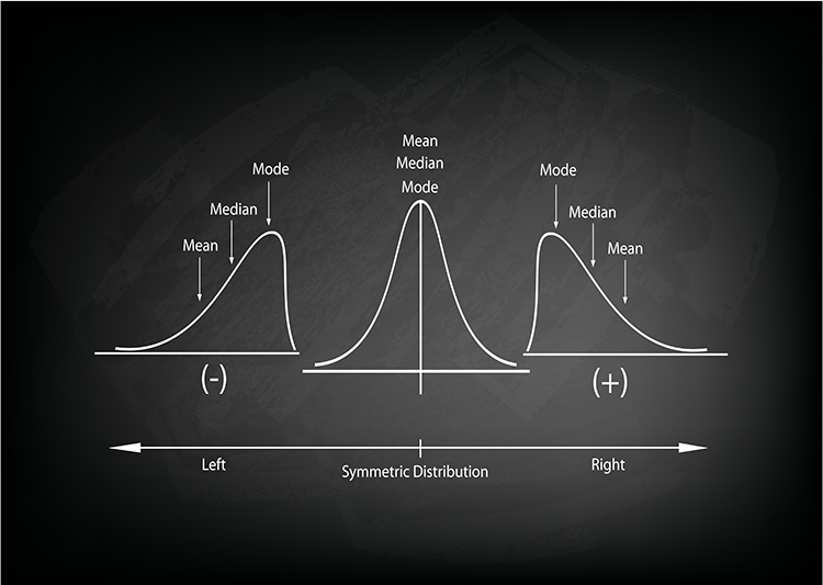
The mean is the arithmetic average and the most commonly reported measure of central tendency. We calculate the mean by adding all values for a variable and then dividing by the number of individuals comprising the sample. The sample mean is represented by X, M, or x̄. The mean's principal limitation is its vulnerability to outliers (extreme scores).
The median divides the sample distribution in half. The median is the middle score or the average of two middle scores. Since the median is unaffected by outliers, statisticians prefer it to the mean when extreme scores are present.
The mode is the most frequent score calculated when there are at least two different sample values. There may be no mode or multiple modes.
Measures of Variability
Statistical measures of variability like the range, standard deviation, the variance, and z-scores index the dispersion in our data. There is no variability [all of these measures are 0] when all sample scores are identical.The range is the difference between the lowest and highest values (or this difference minus 1). For example, for 5, 10, 20, and 25, the range is 20. Since the range is calculated using only two scores in a series, it can be influenced by outliers and cannot show whether data are evenly distributed or clumped together.
The standard deviation is the square root of the average squared deviations from the mean. We represent the sample standard deviation by s or SD.
The standard deviation for a variable is calculated by finding the difference between each value and the mean, squaring each difference, and dividing the sum of squared differences by the number of individuals in the database’s sample. The result is called the variance. The standard deviation is the square root of the variance. It is more commonly used than the variance to show the degree to which individual values deviate from the mean.
For example, for 2, 4, 4, 4, 5, 5, 7, and 9, the standard deviation is the square root of 4, which is 2. When the standard deviation is low, the data points cluster more closely about the mean. When it is high, scores are distributed farther from the mean.
The standard deviation better characterizes the dispersion of scores than the range since it uses all of the data points and is not distorted by outliers.
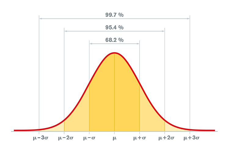
When values are normally distributed, the percentage of scores within 1, 2, and 3 standard deviations from the mean are 68%, 95%, and 99.7%, respectively. Graphic © Peter Hermes Furian/iStockphoto.com.
Clinicians use the standard deviation to determine whether physiological measurements or psychological test scores differ significantly from the standardization sample mean. Check out the YouTube video What Is The Standard Deviation?
The variance is the average squared deviation of scores from their mean and is the square of the standard deviation. For example, for 2, 4, 4, 4, 5, 5, 7, and 9, the variance is 4. A disadvantage of the variance compared with the standard deviation is that it is reported in squared units.
Z-scores, also called standard scores, are especially useful for describing and comparing qEEG findings and delivering neurofeedback.
Using the mean and standard deviation for a variable, a z-score is calculated by subtracting a value from the mean and dividing the difference by the standard deviation. Z-scores have a mean of 0 and a standard deviation of + 1, which quickly shows for any value's distance from the its mean.
If the values are normally distributed in a bell-shaped Gaussian manner, how likely are they to occur if randomly selected from the sample in the database? About 68 percent of database subjects will have a value between +1 and -1 for any variable. Slightly more than 95 percent will have a value between +2 and -2. A value that exceeds + 2 is likely to occur among normally healthy subjects in the database less than 5 percent of the time.
We can quantitatively define the criterion or threshold for what is “normal” in z-scores. Given individual differences, measurement error, and database limitations, these decisions are somewhat aribitrary. For instance, a clinician could define "normal" as a z-score range from -2.00 to +2.00, which would cover 95% of healthy individuals. Z-scores outside of this range would significantly differ from the database sample mean.
Clinicians can covert client data to z-scores and compare them to database norms. Z-scores enjoy great utility because they provide a common unit of measurement for diverse variables. For example, we measure alpha power in μV and coherence from -1.0 to +1.0. However, we can transform both variables to z-scores to visualize their departure from normality using a common metric.
Neurofeedback practitioners use qEEG databases to develop z-score training protocols for their clients. Neurofeedback z-score training software helps identify variables associated with their clients' concerns. The underlying assumption is that reducing extreme values may reduce symptom severity and frequency or improve performance.
A practitioner sets neurofeedback thresholds in z-score units to define how "normal" the EEG value for that variable must be to receive rewarding feedback. The software calculates the value for the EEG variable and converts it to a z-score using database statistics. Variables exceeding a z-score range of -2.00 to +2.00 are likely training candidates since we could expect them to occur less than 5% of the time in a healthy population.
Normal Gaussian Distribution
qEEG normative databases contain means and standard deviations of EEG variables collected from healthy subjects in adjacent age groups during defined assessment conditions (e.g., resting eyes-open, resting eyes-closed). Z-scores allow us to compare an individual’s EEG assessment data with that of the healthy normal database subjects. Z-scores require that EEG variable distrubutions must be Gaussian or normal.What is a Gaussian distribution? This distribution is named for the mathematician Carl Friedrich Gauss (1777-1855). A Gaussian distribution also known as a normal distribution or bell curve, is a continuous probability distribution characterized by its symmetric bell shape, with the mean (μ) at the center and a standard deviation (σ) defining its width. It represents the relationship between a variable, such as alpha power, and the probability or frequency of a specific value for alpha power in a sample of subjects. A Gaussian distribution has a peak in the middle (neither too pointed nor too flat), called the mean or
A Gaussian distribution is symmetric about the mean (μ), meaning that the left and right sides of the curve are mirror images of each other (DeGroot & Schervish, 2012). The mean, median, and mode are all equal to μ. The standard deviation (σ) measures the dispersion or spread of the data. A larger standard deviation indicates a wider distribution, while a smaller standard deviation indicates a narrower distribution.
In a Gaussian distribution, approximately 68% of the data falls within one standard deviation (±σ) of the mean, 95% within two standard deviations (±2σ), and 99.7% within three standard deviations (±3σ). The largest number of scores occur around the mean. Very high or very low scores occur less frequently.
The Relationship Between Gaussian and z-Distributions
A z-distribution, also known as the standard normal distribution, is a special case of the Gaussian distribution. The z-distribution has a mean (μ) of 0 and a standard deviation (σ) of 1. In other words, a z-distribution is a Gaussian distribution with its parameters set to μ = 0 and σ = 1.The relationship between the z-distribution and the Gaussian distribution is often used for standardization in statistical analyses. By transforming the data from a general Gaussian distribution to a z-distribution, we can compare data from different distributions and apply standardized statistical methods. A z-score represents the number of standard deviations that a specific data point is from the mean of the distribution. This transformation is useful when working with statistical hypothesis tests, confidence intervals, and other inferential techniques that rely on the properties of the standard normal distribution.
Data Transformation
When data are not normally distributed, we can use linear transformations (e.g., log10) to normalize them (Thatcher, North, & Biver, 2005a).Gaussian Sensitivity
Gaussian sensitivity describes the degree of uncertainty (or accuracy and “certainty”) a dataset possesses (Thatcher et al., 2003, p. 101). In the forensic context, Gaussian sensitivity is important because of its relationship to an instrument’s measurement error, which is one of the Daubert standards (Daubert v Merrell Dow, 1993).Thatcher et al. (2005) define sensitivity as the difference between two data distributions: an ideal Gaussian and EEG sample values. This discrepancy should be as small as possible.
Sensitivity refers to the proportion of true positive cases among the individuals who actually have the disease or condition. In other words, it measures the test's ability to correctly identify those with the disease. A highly sensitive test will have a low rate of false negatives (i.e., cases where the test fails to detect the disease when it is present).
Specificity, on the other hand, refers to the proportion of true negative cases among the individuals who do not have the disease or condition. It measures the test's ability to correctly identify those without the disease. A highly specific test will have a low rate of false positives (i.e., cases where the test mistakenly indicates the presence of the disease when it is not present).
Medical tests and EEG measurements should have high sensitivity and specificity (Altman & Bland, 1994; McNamara & Martin, 2018; Parikh et al., 2008).
Normal Distributions
Normally distributed EEG database values minimize error in estimating population EEG values (Thatcher, Walker, Biver, North, & Curtin, 2003). Kurtosis and skewness are two statistical measures that describe the shape of a distribution, specifically deviations from a Gaussian (normal) distribution.Kurtosis
Kurtosis is a measure of the "tailedness" or the concentration of data in the tails of a distribution. A distribution with high kurtosis has more data in the tails, resulting in a more peaked and heavy-tailed shape compared to a Gaussian distribution.There are three primary types of kurtosis: mesokurtic, leptokurtic, and platykurtic. Each represents a different degree of concentration of data in the tails relative to a Gaussian distribution.
Mesokurtic
A mesokurtic distribution has a kurtosis value that is equal to that of a Gaussian distribution, which is 3. When reporting excess kurtosis (kurtosis value minus 3), mesokurtic distributions have an excess kurtosis value of 0. Mesokurtic distributions have a similar shape to Gaussian distributions, with a moderate concentration of data in the tails and a "normal" peakedness. Most of the real-world data that are normally distributed are mesokurtic (Westfall, 2014).
Leptokurtic
A leptokurtic distribution has a kurtosis value greater than 3 (positive excess kurtosis). Leptokurtic distributions are characterized by more data in the tails and a more peaked shape compared to a Gaussian distribution. They have heavy tails, which means there is a higher likelihood of extreme values or outliers. These distributions might require special attention in statistical analyses, as they could lead to biased estimators and inflated Type I error rates when the assumption of normality is violated (DeCarlo, 1997).
Platykurtic
A platykurtic distribution has a kurtosis value less than 3 (negative excess kurtosis). Platykurtic distributions have fewer data points in the tails and a more rounded shape compared to a Gaussian distribution. They have light tails, which means there is a lower likelihood of extreme values or outliers. In some cases, these distributions may be more appropriate for analyses that assume homoscedasticity or constant variance across the distribution (Balanda & MacGillivray, 1988).
Understanding kurtosis is important for statistical analysis and data interpretation.
1. Assumption of normality
Many statistical tests and models assume that the data are normally distributed. A distribution with non-zero excess kurtosis deviates from the normal distribution in terms of its "tailedness." Understanding kurtosis can help identify when the normality assumption is violated, which may lead to incorrect inferences or conclusions. This information enables researchers to choose appropriate transformations, methods, or models to better analyze and interpret the data (DeCarlo, 1997).
2. Outliers and extreme values
High kurtosis, particularly in leptokurtic distributions, indicates a higher likelihood of extreme values or outliers in the data. These extreme values can have a significant impact on the estimation of parameters, statistical tests, and model performance. Being aware of the kurtosis can help researchers decide whether to use robust statistical techniques that are less sensitive to the presence of outliers or whether to investigate the potential causes of these extreme values (Balanda & MacGillivray, 1988).
3. Homoscedasticity assumption
In some statistical models, such as linear regression, the assumption of homoscedasticity (constant variance) is made. Platykurtic distributions, which have a lower concentration of data points in the tails, may be more appropriate for analyses that assume homoscedasticity. Understanding kurtosis can help researchers evaluate whether this assumption is reasonable for their data (Balanda & MacGillivray, 1988).
4. Data transformation
In some cases, data with high or low kurtosis may benefit from transformations (e.g., log, square root, or Box-Cox transformations) to achieve a more Gaussian-like distribution, which may improve the performance of statistical tests and models that assume normality. Understanding kurtosis can inform the choice of appropriate transformations (Templeton, 2011).
Skewness
Skewness is a measure of a distribution's asymmetry. There are three primary types of skewness: symmetric (no skew), positively skewed, and negatively skewed. Each type represents a different degree of asymmetry in the distribution relative to a Gaussian (normal) distribution, which is symmetric and has a skewness of 0.Symmetric (No Skew)
A symmetric distribution has a skewness value of 0, indicating that there is no asymmetry in the distribution. The tails on both sides of the distribution are equal, and the mean, median, and mode of the distribution coincide. Gaussian distributions are an example of symmetric distributions. In real-world data, if a distribution is approximately symmetric, it suggests that the data points are evenly distributed around the central tendency (Joanes & Gill, 1998).
Positively Skewed
A positively skewed distribution has a skewness value greater than 0. In this case, the right tail of the distribution is longer or more stretched out than the left tail. Positively skewed distributions are also referred to as right-skewed distributions. In a positively skewed distribution, the mean is greater than the median, which is greater than the mode. These distributions often occur when data points have a lower bound (e.g., income, age at death, or exam scores) but no upper bound, leading to a concentration of data points at the lower end and a longer tail at the upper end (Bulmer, 1979).
Negatively Skewed
A negatively skewed distribution has a skewness value less than 0. In this case, the left tail of the distribution is longer or more stretched out than the right tail. Negatively skewed distributions are also referred to as left-skewed distributions. In a negatively skewed distribution, the mean is less than the median, which is less than the mode. These distributions often occur when data points have an upper bound (e.g., a percentage between 0 and 100) but no lower bound, leading to a concentration of data points at the upper end and a longer tail at the lower end (Bulmer, 1979).
Understanding skewness is important because it can affect the choice of statistical methods or transformations used for data analysis. Skewed data may require non-parametric tests, transformations, or the use of robust estimators that are less sensitive to the presence of outliers.
We can calculate kurtosis and skewness to see how much an EEG score distribution deviates from a normal distribution. When there is significant deviation, we can mathematically transform these values, for example, with a log10 transformation, to better satisfy parametric test assumptions and reduce errors of estimate. When linear transformations fail to meet test assumptions, we must use their nonparametric counterparts.
Percentiles
Percentiles are a measure used in statistical analysis to describe the relative standing of a data point within a dataset. A percentile indicates the percentage of data points in the dataset that are below a specific value. Percentiles are particularly useful for understanding the distribution of data, comparing data points across different datasets, and interpreting non-normally distributed data (Hyndman & Fan, 1996).To interpret percentiles, consider a data point's percentile rank. For example, if a data point has a 70th percentile rank, it means that 70% of the data points in the dataset are equal to or below that value, while the remaining 30% are above it. Percentiles can be used to identify various data points within the distribution, such as the median (50th percentile), quartiles (25th, 50th, and 75th percentiles), and other percentiles that partition the data into equal segments (Wilcox, 2012).
Percentiles are important in statistical analysis for several reasons:
1. Distribution description
Percentiles provide a way to describe the distribution of data without making assumptions about its shape. They can be used to characterize the central tendency, dispersion, and tail behavior of a distribution, regardless of whether it is normal, skewed, or has heavy tails (Hyndman & Fan, 1996).
2. Non-parametric analysis
Percentiles are especially valuable for non-parametric analyses, which do not rely on assumptions about the underlying distribution. Non-parametric tests, such as the Mann-Whitney U test or the Kruskal-Wallis test, utilize percentile ranks to compare groups or samples without assuming normality (Conover, 1999).
3. Comparison across EEG datasets
Percentiles enable comparison of data points across different datasets or populations with different scales or units of measurement. For example, standardized test scores are often reported as percentiles, allowing for a comparison of students' performance across different tests or educational systems (Feinberg & Wainer, 2014).
4. Robustness
Percentiles are robust to the presence of outliers, as they are not heavily influenced by extreme values. This makes them particularly useful for summarizing and comparing data that may have skewed or heavy-tailed distributions (Wilcox, 2012).
Defining Normal EEG Values
The logic behind using z-scores to define normal values lies in the properties of a standard normal distribution, which is a Gaussian distribution with a mean of 0 and a standard deviation of 1. When data are transformed into z-scores, they become comparable to the standard normal distribution, allowing for the interpretation of individual data points in terms of their relative position within the distribution (DeCarlo, 1998).Under the standard normal distribution, approximately 68% of the data falls within one standard deviation from the mean (i.e., z-scores between -1 and 1), 95% of the data falls within two standard deviations from the mean (i.e., z-scores between -2 and 2), and 99.7% of the data falls within three standard deviations from the mean (i.e., z-scores between -3 and 3). This is known as the empirical rule or the 68-95-99.7 rule (Kwak & Kim, 2017).
Using z-scores, normal values can be defined as those that fall within a certain range of standard deviations from the mean. For instance, if we consider values within two standard deviations from the mean as "normal," then any data point with a z-score between -2 and 2 would be considered normal, while data points with z-scores below -2 or above 2 would be considered unusual or extreme. The specific range of z-scores used to define normal values may vary depending on the context or the specific application (Gravetter & Wallnau, 2016).
A database user could set the normal range as any z-score between -2.0 and +2.0 based on the knowledge that about 95 percent of z-scores for subjects in the qEEG normative database will have values that fall in that range. Such a definition, however, is somewhat arbitrary, with another user perhaps choosing to define normal as any z-score between -1.5 and +1.5 to narrow the range of what is considered normal and expand the range of what is considered abnormal (i.e., z-scores less than -1.5 or greater than +1.5). z-scores outside the selected range are then defined as being statistically significant, unlikely to have occurred by chance among normally healthy individuals, unexpected, or “abnormal.”
Alpha Levels and Probability Values
Alpha levels, also known as significance levels, are a critical component of hypothesis testing in statistical analysis. An alpha level is a predetermined threshold, usually denoted as α, used to determine whether the results of a hypothesis test are statistically significant. It represents the probability of making a Type I error, which occurs when the null hypothesis is rejected when it is, in fact, true (Cohen, 1994).Neurofeedback and qEEG providers utilize alpha levels (e.g., frequently p = 0.05) to define when EEG variables significantly deviate from normative database values to be considered abnormal.
The role of alpha levels in statistical analysis is to provide a benchmark for deciding whether to reject or fail to reject the null hypothesis. When performing a hypothesis test, a test statistic is calculated, and its corresponding probability value (p-value) is compared to the chosen alpha level. If the p-value is less than the alpha level, the null hypothesis is rejected, and the results are considered statistically significant. If the p-value is equal to or greater than the alpha level, the null hypothesis is not rejected, and the results are considered not statistically significant (Levin & Fox, 2018).
There is some disagreement among statisticians and researchers regarding whether to reject the null hypothesis if a test statistic is equal to the alpha level. A p-value equal to the alpha level represents a borderline case, where the evidence against the null hypothesis is right at the threshold of what is considered statistically significant. Some researchers may see this as sufficient evidence to reject the null hypothesis, while others may consider it inconclusive (Haller & Krauss, 2002).
In practice, the choice of whether to reject the null hypothesis when the p-value is equal to the alpha level often depends on the specific context, the consequences of Type I and Type II errors, and the researcher's own judgment. It is important to note that hypothesis testing is just one aspect of statistical analysis, and the interpretation of results should also consider effect sizes, confidence intervals, and other relevant information (Cumming, 2014).
Commonly used alpha levels are 0.05, 0.01, and 0.001, indicating a 5%, 1%, or 0.1% probability of making a Type I error, respectively. A lower alpha level corresponds to a more stringent threshold for statistical significance and a lower probability of making a Type I error. The choice of alpha level depends on the specific context and the desired balance between Type I and Type II errors (Cohen, 1994).
Alpha levels are important in statistical analysis for several reasons:
1. Decision-making
Alpha levels provide a systematic and objective way to make decisions about the null hypothesis, facilitating the interpretation and communication of results (Levin & Fox, 2018).
2. Control of Type 1 errors
By setting an alpha level, researchers control the probability of making a Type I error, which can help minimize the likelihood of false-positive findings (Cohen, 1994).
3. Reproducibility and comparability
The use of standard alpha levels, such as 0.05, allows for the comparison and reproducibility of findings across different studies and disciplines (Nuzzo, 2014).
4. Balancing errors
The choice of alpha level helps researchers balance the risks of Type I and Type II errors, depending on the specific context and consequences associated with each type of error (Cohen, 1994).
Correlation Coefficients
Correlation is a statistical measure that describes the strength and direction of the relationship between two variables. It helps researchers understand how variables change together and can be used to make predictions.Correlation coefficients are used to calculate EEG measures such as coherence and comodulation. Coherence and comodulation are measures used in the analysis of EEG data to quantify the relationship between neural oscillations recorded at different locations on the scalp. They provide insights into the functional connectivity and information flow between brain regions during cognitive processing or resting state.
Coherence is a frequency-domain measure that quantifies the consistency of the phase relationship between two signals across time. It ranges from 0 (no consistency) to 1 (perfect consistency) and is based on cross-spectral density and auto-spectral density. Coherence is particularly useful for analyzing oscillatory activity in the brain, such as during cognitive tasks or sleep.
Comodulation, also known as cross-frequency coupling, measures the interaction between oscillations at different frequency bands. It helps to understand the hierarchical organization of brain oscillations and their role in information processing. Comodulation can be further divided into amplitude-amplitude, phase-phase, and phase-amplitude couplings.
Correlation, in the context of EEG analysis, refers to the linear relationship between the amplitudes of two signals. It is a time-domain measure that ranges from -1 (perfect negative correlation) to 1 (perfect positive correlation). Correlation does not capture the frequency-specific information or phase relationships between signals, which are critical for understanding neural dynamics.
Coherence and comodulation differ in their focus on the frequency domain and the type of relationship they measure. While coherence quantifies the consistency of phase relationships within a specific frequency band, comodulation measures interactions between oscillations at different frequencies. Both coherence and comodulation can provide complementary information about brain connectivity, with each offering unique insights into the functional organization of the brain.
Linear and Nonlinear Correlations
In linear correlation, there is a straight-line relationship between two variables. The variables increase or decrease together in a consistent and proportional manner. The most commonly used measure of linear correlation is the Pearson correlation coefficient (r), which ranges from -1 to 1. A positive value indicates a direct relationship (both variables increase together), a negative value indicates an inverse relationship (one variable increases as the other decreases), and a value of zero indicates no linear relationship.In nonlinear correlation, the relationship between two variables is not linear but follows a curve or other pattern. It is often more complex and harder to describe mathematically. The most common measure of nonlinear correlation is the Spearman rank correlation coefficient (ρ), which is based on the ranks of the data rather than their actual values.
Correlation Does Not Prove Causation
Correlation indicates a relationship between two variables, but it does not prove that one variable causes the other. There are several reasons for this:1. Confounding variables
A third variable, not considered in the analysis, might be causing the observed correlation.
2. Reverse causation
It is possible that the direction of causation is reversed, meaning that the presumed cause is actually the effect and vice versa.
3. Coincidence
The observed correlation could be the result of chance, with no real relationship between the variables.
4. Bidirectional causation
Both variables might influence each other, making it difficult to determine the true cause and effect.
Overview of qEEG
Normative Databases
EEG normative databases quantify EEG variables such as amplitude, power, coherence, and phase using EEG samples obtained from healthy normal subjects. These variables are calculated for typical EEG bands or single-hertz bins and all electrode sites and their connections. Values for Brodmann Areas, anatomical structures, regions of interest, and their various connections may also be included.The EEG of an individual client can then be compared to the normative database to see if the client’s EEG deviates to any significant degree from normal. Those EEG variables that deviate from normal may then become targets for neurofeedback training if there is reason to think they are related to the client’s concerns or symptoms.
Normative EEG databases are constructed by selecting data from healthy normal subjects from several age ranges. Subjects are selected for age ranges across the life span because the normal value of EEG variables change during maturation. For example, the amplitude of the eyes-closed delta range decreases as a child ages. Subjects are also selected to exclude conditions that might affect the EEG, such as a diagnosed mental health condition, addiction, or neurological disorder.
Databases usually include samples from eyes-open and eyes-closed conditions because the normal EEG differs under such conditions. Some databases may also include data acquired during cognitive tasks, for example, related to attention, memory, or problem-solving.
The values of the EEG variables for the database’s subjects are usually transformed into z-scores that are distributed in a bell-like Gaussian curve. In this “normal curve,” most values cluster around the average. Values that are greater than or less than average occur less frequently the more they diverge from the average value. Z-scores are calculated by subtracting an individual’s raw score from the average score of the healthy normal sample and then dividing the remainder by the standard deviation of the sample.
The standard deviation is simply a measure of how variable the data are. A z-score is expressed in standard deviation units of how far a score deviates from the average. When the raw data are transformed into z-scores, a z-score of 0 is the average. Below-average raw scores have a negative z-score, while above-average raw scores have a positive z-score. Approximately 68% of a group’s raw scores will have z-scores between +1 and -1 standard deviations from 0 (i.e., within + 1 SD). About 95% of the group will have z-scores between +2 and -2 standard deviations. Graphic © Peter Hermes Furian/iStockphoto.com.
When a practitioner collects EEG data from an individual client and analyzes their data with a normative database, they calculate the client’s average value of the variable of interest from artifact-free data. For example, after removing artifacts, the practitioner calculates the client’s average number of microvolts in the alpha range with eyes closed.
The number for the client is then compared to the average number of microvolts that the database’s healthy normal subjects of a similar age have with their eyes closed. That difference is divided by the standard deviation of eyes-closed microvolts of alpha for similar-aged normal subjects to produce a z-score.
If the resulting z-score for the client is between +2 and -2, the practitioner may consider the client’s eyes- closed alpha activity to be within the normal range. If the client’s z-score is less than -2, it is significantly deficient or lower than normal. If the client’s z-score is more than +2, it is excessive or significantly greater than normal. The range of z-scores that encompasses “normal” is somewhat arbitrary. For instance, some practitioners use a + 1.5 SD range, and others use a + 2 SD range.
Several companies offer normative databases for clinical and research applications. These include Applied NeuroScience, Human Brain Institute, and qEEG Pro, among others.
Glossary
amplitude: the strength of the EEG signal measured in microvolt or picowatts.
artifact: false signals like 50/60Hz noise produced by line current.
alpha blocking: alpha blocking normally occurs when eyes have just been opened. Arousal and specific forms of cognitive activity may reduce alpha amplitude or eliminate it while increasing EEG power in the beta range.
alpha response: increased alpha amplitude.
alpha rhythm: 8-12-Hz activity that depends on the interaction between rhythmic burst firing by a subset of thalamocortical (TC) neurons linked by gap junctions and rhythmic inhibition by widely distributed reticular nucleus neurons. Researchers have correlated the alpha rhythm with relaxed wakefulness. Alpha is the dominant rhythm in adults and is located posteriorly. The alpha rhythm may be divided into alpha 1 (8-10 Hz) and alpha 2 (10-12 Hz).
alpha spindles: trains of alpha waves that are visible in the raw EEG and are observed during drowsiness, fatigue, and meditative practice.
alpha-theta training: protocol to slow the EEG to the 6-9 Hz crossover region while maintaining alertness.
amplitude: the strength of the EEG signal measured in microvolts or picowatts, and as seen in the peak-to-trough height of EEG waves.
beta rhythm: 12-38-Hz activity associated with arousal and attention generated by brainstem mesencephalic reticular stimulation that depolarizes neurons in the thalamus and cortex. The beta rhythm can be divided into multiple ranges, often defined as: beta 1 (12-15 Hz), beta 2 (15-18 Hz), beta 3 (18-25 Hz), and beta 4 (25-38 Hz).
beta spindles: trains of spindle-like waveforms with frequencies that can be lower than 20 Hz but more often fall between 22 and 25 Hz. They may signal ADHD, especially with tantrums, anxiety, autistic spectrum disorders (ASD), epilepsy, and insomnia.
bipolar (sequential) montage: a recording method that uses two active scalp electrodes and a common reference.
clinical database approach: using information such as ratios, measures of differences from one location to another, peak frequency information, maximum voltage, minimum voltage, and other metrics to determine how the client's EEG differs from expected characteristics and what can be done to restore optimal functioning.
common-mode rejection (CMR): using a differential amplifier, eliminating simultaneous, in-phase signals that occur at the two electrode sites.
cross-frequency synchronization (CFS): a mechanism in which waves of one type of frequency, such as beta or gamma, occur synchronously with the wave patterns of slower frequencies such as delta, theta, or alpha. These are often described as nested rhythms.
default mode network (DMN): a cortical network of sites located in frontal, temporal, and parietal regions that is most active during introspection and daydreaming and relatively inactive when pursuing external goals.
delta rhythm: 0.05-3 Hz oscillations generated by thalamocortical neurons during stage 3 sleep.
depolarization: to make the membrane potential less negative by making the inside of the neuron less negative with respect to its outside.
EEG activity: electrical activity of the cortex.
EEG artifacts: noncerebral electrical activity in an EEG recording can be divided into physiological and exogenous artifacts.
electrode: a specialized conductor that converts biological signals like the EEG into currents of electrons.
frequency (Hz): the number of complete cycles that an AC signal completes in a second, usually expressed in hertz.
gamma rhythm: EEG activity frequencies above 30 or 35 Hz. Frequencies from 25-70 Hz are called low gamma, while those above 70 Hz represent high gamma.
hertz (Hz): unit of frequency measured in cycles per second.
International 10-10 system: a modified combinatorial system for electrode placement that expands the 10-20 system to 75 electrode sites to increase EEG spatial resolution and improve detection of localized evoked potentials.
International 10-20 system: a standardized procedure for 21 recording and one ground electrode on adults.
Joint Frequency Time Analysis (JFTA): an analytical procedure that plots the spectral distribution of signal power over time.
magnetoencephalography (MEG): a noninvasive functional imaging technique that uses SQUIDs (superconducting quantum interference devices) to detect the weak magnetic fields generated by neuronal activity.
magnetic resonance imaging (MRI): a noninvasive imaging technique that uses strong magnetic fields and bursts of RF energy to construct highly detailed images of the living brain.
microvolt (μV): the unit of amplitude (signal strength) that is one-millionth of a volt.
mirror neuron system: network of locations associated with what might be termed learning by observation, mimicry, or imitation.
movement artifact: voltages caused by client movement or the movement of electrode wires by other individuals.
mu rhythm: 7-11-Hz waves that resemble wickets and appear as several-second trains over central or centroparietal sites (C3 and C4).
normative database approach: comparing a client's EEG to a "normal" sample, identifying variations, and selecting training locations and frequencies.
polarization: to make the membrane potential more negative by making the inside of the neuron more negative with respect to its outside.
nystagmus: an involuntary rhythmic side-to-side, up and down, or circular motion of the eyes that occurs with a variety of conditions.
positron emission tomography (PET): a functional imaging technique that injects radioactive chemicals into the brain's circulation to measure brain activity.
posterior dominant rhythm (PDR): the highest-amplitude frequency detected at the posterior scalp when eyes are closed.
power: amplitude squared and may be expressed as microvolts squared or picowatts/resistance.
Quantitative EEG (qEEG): digitized statistical brain mapping using at least a 19-channel montage to measure EEG amplitude within specific frequency bins.
reference electrode: an electrode placed on the scalp, earlobe, or mastoid.
reticular nucleus of the thalamus (TRN): GABAergic thalamic neurons that modulate signals from other thalamic nuclei and do not project to the cortex. Also called the nucleus reticularis of the thalamus (NRT).
sensorimotor rhythm (SMR): EEG rhythm that ranges from 12-15 Hz and is located over the sensorimotor cortex (central sulcus). The waves are synchronous. The sensorimotor rhythm is associated with the inhibition of movement and reduced muscle tone. The SMR is generated by "ventrobasal relay cells in the thalamus and thalamocortical feedback loops."
single photon emission computerized tomography (SPECT): a functional imaging technique that uses gamma rays to create three-dimensional and slice images of cerebral blood flow averaged over several minutes.
slow cortical potential (SCP): slow event-related direct-current shifts of the electroencephalogram. Cortical potential shifts precede the depolarization of large cortical assemblies. The negative shift reflects the actions of gap junction cells. That shift reduces the excitation threshold of pyramidal neurons, leading to increased firing or depolarization of large assemblies of pyramidal neurons.
symptom-matching approach: a "decision tree" approach using workbooks or guides that provide an "if this, then do that" format with a series of steps to be followed if initial interventions do not provide adequate relief.
synchrony: the coordinated firing of pools of neurons due to pacemakers and mutual coordination.
thalamic-cortical relay (TCR) system: the primary pathway for determining which areas of the cortex receive each type of sensory input.
theta/beta ratio: the ratio between 4-7 Hz theta and 13-21 Hz beta, measured as amplitude squared most typically along the midline and generally in the anterior midline near the 10-20 system location Fz.
theta rhythm: 4-8-Hz rhythms generated by a cholinergic septohippocampal system that receives input from the ascending reticular formation and a noncholinergic system that originates in the entorhinal cortex, which corresponds to Brodmann areas 28 and 34 at the caudal region of the temporal lobe.
vertex (Cz): the intersection of imaginary lines drawn from the nasion to inion and between the two preauricular points in the International 10-10 and 10-20 systems.
waveform: the shape and form of an EEG signal.
TEST YOURSELF ON CLASSMARKER
Click on the ClassMarker logo below to take a 10-question exam over this entire unit.

REVIEW FLASHCARDS ON QUIZLET PLUS
Click on the Quizlet Plus logo to review our chapter flashcards.

Visit the BioSource Software Website
BioSource Software offers Functional Neuroanatomy, which reviews critical behavioral networks, and qEEG100, which provides extensive multiple-choice testing over the IQCB Blueprint.

Assignment
Now that you have completed this unit, describe how you explain the qEEG to your clients. Which training apporach do you use. Why?
References
Ancoli, S., & Kamiya, J. (1978). Methodological issues in alpha biofeedback training. Biofeedback and Self-Regulation, 3(2). 159-183. https://doi.org/0.1007/BF00998900
Arns, M., de Ridder, S., Strehl, U., Breteler, M., & Coenen, A. (2009). Efficacy of neurofeedback treatment in ADHD: The effects on inattention, impulsivity and hyperactivity: A meta-analysis. Clinical EEG and neuroscience, 40(3), 180–189. https://doi.org/10.1177/155005940904000311
Berger, H. (1929). Über das Elektrenkephalogramm des Menschen. Archiv f. Psychiatrie, 87, 527–570.
Britton, J. W., Frey, L. C., Hopp, J. L., Korb, P., Koubeissi, M. Z., Lievens, W. E., Pestana-Knight, E. M., & St. Louis. E. K., E. K. St. Louis, L. C. Frey (Eds.) (2016). Electroencephalography (EEG): An introductory text and atlas of normal and abnormal findings in adults, children, and infants. American Epilepsy Society.
Cohen, M. P. (2020). Neurofeedback 101: Rewiring the brain for ADHD, anxiety, depression and beyond (without medication). Center from Brain Training.
Cox, C. L., Huguenard, J. R., & Prince, D. A. (1997). Nucleus reticularis neurons mediate diverse inhibitory effects in thalamus. Proceedings of the National Academy of Sciences, 94(16), 8854-8859. https://doi.org/10.1073/pnas.94.16.8854
Davey, C. G., & Harrison, B. J. (2018). The brain's center of gravity: How the default mode network helps us to understand the self. World Psychiatry: Official Journal of the World Psychiatric Association (WPA), 17(3), 278-279. https://doi.org/10.1002/wps.20553
Demos, J. N. (2019). Getting started with neurofeedback (2nd ed.). W. W. Norton & Company.
Fisch, B. J. (1999). Fisch and Spehlmann's EEG primer (3rd ed.). Elsevier.
ISNR Board of Directors (2010). What is neurofeedback? Retrieved from https://isnr.org/what-is-neurofeedback.
Kamiya, J. (1961). Behavioral, subjective, and physiological aspects of drowsiness and sleep. In D. W. Fiske, & S. R. Maddi (Eds.). Functions of varied experience. Dorsey Press.
Kamiya, J. (1962). Conditioned discrimination of the EEG alpha rhythm in Humans. Abstract presented at the Western Psychological Association meeting.
Kamiya, J. (1968). Conscious control of brain waves. Psychology Today, 1, 56-63.
Kamiya, J. (1969). Operant control of the EEG alpha rhythm and some of its reported effects on consciousness. In C. Tart (Ed.), Altered states of consciousness. John Wiley and Sons.
Nicholson, A. A., Densmore, M., MicKinnon, M. C., Neufeld, R. W. J., Frewen, P. A. Théberge, J., Jetly, R., Richardson, J. D., & Lanius, R. A. (2019). Machine learning multivariate pattern analysis predicts classification of posttraumatic stress disorder and its dissociative subtype: A multimodal neuroimaging approach. Psychol Med, 49(12), 2049-2059. https://doi.org/10.1017/S003329171800286
Nicholson, A. A., Ros, T., Densmore, M., Frewen, P. A., Neufeld, R. W. J., Théberge, J., Jetly, R., & Lanius, R. A. (2020). A randomized, controlled trial of alpha-rhythm EEG neurofeedback in posttraumatic stress disorder: A preliminary investigation showing evidence of decreased PTSD symptoms and restored default mode and salience network connectivity using fMRI. Neuroimage Clin., 28, 102490. https://doi.org/10.1016/j.nicl.2020.102490
Nicholson, A. A., Ros, T., Jetly, R., & Lanius, R. (2020). Regulating posttraumatic stress disorder symptoms with neurofeedback: Regaining control of the mind. Journal of Military Veteran and Family Health 6(S1), 3-15. https://doi.org/10.3138/jmvfh.2019-0032
Othmer, S. (2006). Protocol guide for neurofeedback clinicians. EEG Info, Inc.
Peniston, E. G., & Kulkosky, P. J. (1989). Alpha-theta brain wave training and beta-endorphin levels in alcoholics. Alcoholism, Clinical and Experimental Research, 13, 271–279. https://doi.org/10.1111/j.1530-0277.1989.tb00325.x
Peniston, E. G., & Kulkosky, P. J. (1990). Alcoholic personality and alpha-theta brainwave training. Medical Psychotherapy, 3, 37–55.
Pfister, H., Kaynig, V., Botha, C. P., Bruckner, S., Dercksen, V., & Hege, H.-C. (2012). Visualization in connectomics. Mathematics and Visualization, 37. https://doi.org/10.1007/978-1-4471-6497-5_21
Scott, W., & Kaiser, D. (2005). Effects of an EEG biofeedback protocol on a mixed substance abusing population. The American Journal of Drug and Alcohol Abuse, 31(3), 455-469. https://doi.org/10.1081/ada-200056807
Swingle, P. G. (2008). Biofeedback for the brain: How neurotherapy effectively treats depression, ADHD, autism, and more. Rutgers University Press.
Swingle, P. G. (2015). Adding neurotherapy to your practice: Clinician's guide to the ClinicalQ, neurofeedback, and braindriving. Springer International Publishing. https://doi.org/10.1007/978-3-319-15527-2
Thompson, M., & Thompson, L. (2015). The biofeedback book: An introduction to basic concepts in applied psychophysiology (2nd ed.). Association for Applied Psychophysiology and Biofeedback.
Weise, R., von Mengden, I., Glos, M., Garcia, C., & Penzel, T. (2013). P 153. Influence of transcranial slow oscillation current stimulation (tSOS) on EEG, sleepiness and alertness. Clinical Neurophysiology, 124(10), e137. https://doi.org/10.1016/j.clinph.2013.04.230