IQCB Blueprint Coverage

This unit addresses III. Technical (3 Hours). The competent clinical neurophysiologist must acquire knowledge of electronics and instrumentation related to the EEG and ERPs.




This unit covers:
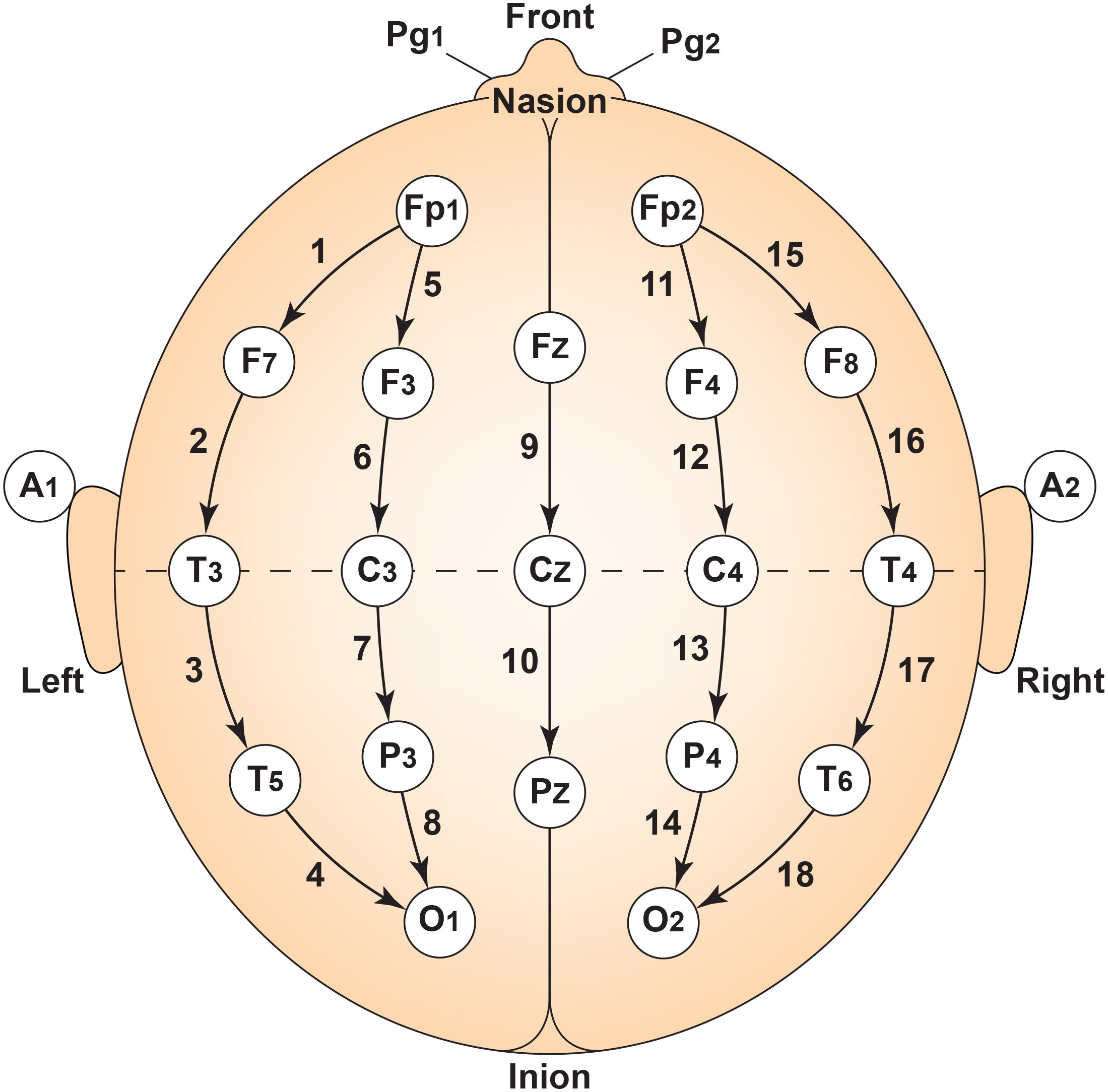
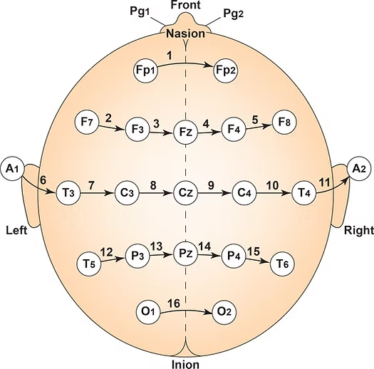
A. Topographical Representation of the EEG
B. Electrodes and Acquisition Systems
C. Instrumentation (Acquisition and Review Parameters/Settings)
D. Montages
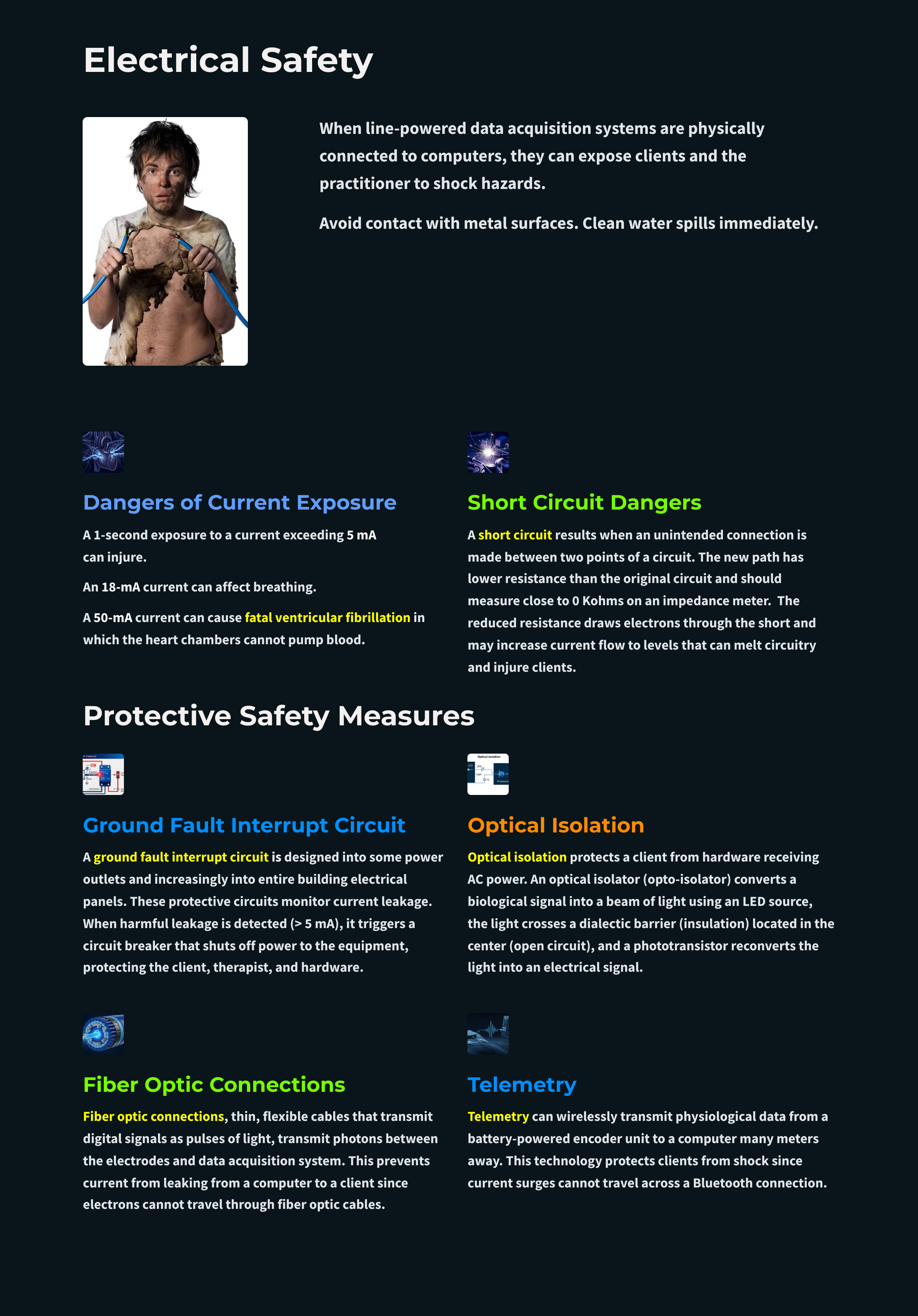
E. Electrical/Clinical Safety

A. Topographical representation of the EEG

Please click on the podcast icon below to hear a full-length lecture over Section A.



Quantitative electroencephalography (qEEG) involves the mathematical analysis of the EEG signals to extract quantitative information about the brain's electrical activity. One crucial aspect of qEEG is the topographical representation, which provides a spatial map of EEG activity across the scalp. Topographical mapping is essential for visualizing the distribution and intensity of electrical potentials, facilitating the identification of regional brain activity patterns and abnormalities.

The raw EEG signals undergo preprocessing steps, including filtering, artifact removal, and segmentation into epochs. This preprocessing ensures that the signals are clean and ready for further analysis. The signals are then subjected to spectral analysis, usually via Fourier Transform, to decompose them into their constituent frequency bands (e.g., delta, theta, alpha, beta, gamma). Each frequency band is associated with different brain states and functions.

The processed data from each electrode are used to create a spatial representation of brain activity. This involves interpolating the values between electrodes to generate a continuous map. Topographical maps can be color-coded to represent the intensity of electrical activity at different scalp locations. These maps visually display how specific frequency bands or other EEG metrics (e.g., power, coherence) are distributed across the scalp.

Topographical EEG maps are used in clinical settings to identify and localize abnormal brain activity associated with various neurological conditions, such as epilepsy, brain injuries, and psychiatric disorders. In research, these maps help study brain function and connectivity, investigate neural mechanisms underlying cognitive processes, and assess interventions' effects.

The benefits of topographical mapping are enhanced visualization, brain activity localization, and diagnostic accuracy.

Enhanced visualization: Topographical representation provides an intuitive and detailed visualization of brain activity, making it easier for clinicians and researchers to interpret complex EEG data.

Brain function localization: Topographical EEG can help localize specific brain functions and detect abnormalities in particular regions by mapping the spatial distribution of electrical activity.

Improved diagnostic accuracy: In clinical practice, topographical maps enhance the accuracy of diagnosing neurological conditions by revealing subtle abnormalities that may not be apparent in raw EEG traces.

The Development of Z-Score Training

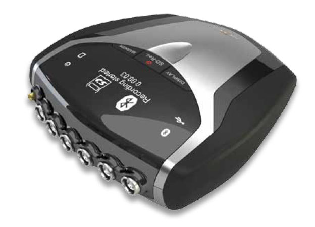
To meet the need for z-score training, Robert Thatcher, developer of the NeuroGuide database, in cooperation with Thomas Collura of BrainMaster Technologies, developed Live Z-Score Training (LZT). Beginning in about 1996 (Thatcher et al., 2019), they started with a simple 1- or 2-channel approach that quickly developed into a 4-channel system for training clients by providing real-time information about how closely their EEG matched a database of age-matched typical controls. There were approximately 72 variables available within the Thatcher database, including power, relative power, phase and coherence values, and more for the standard EEG frequencies.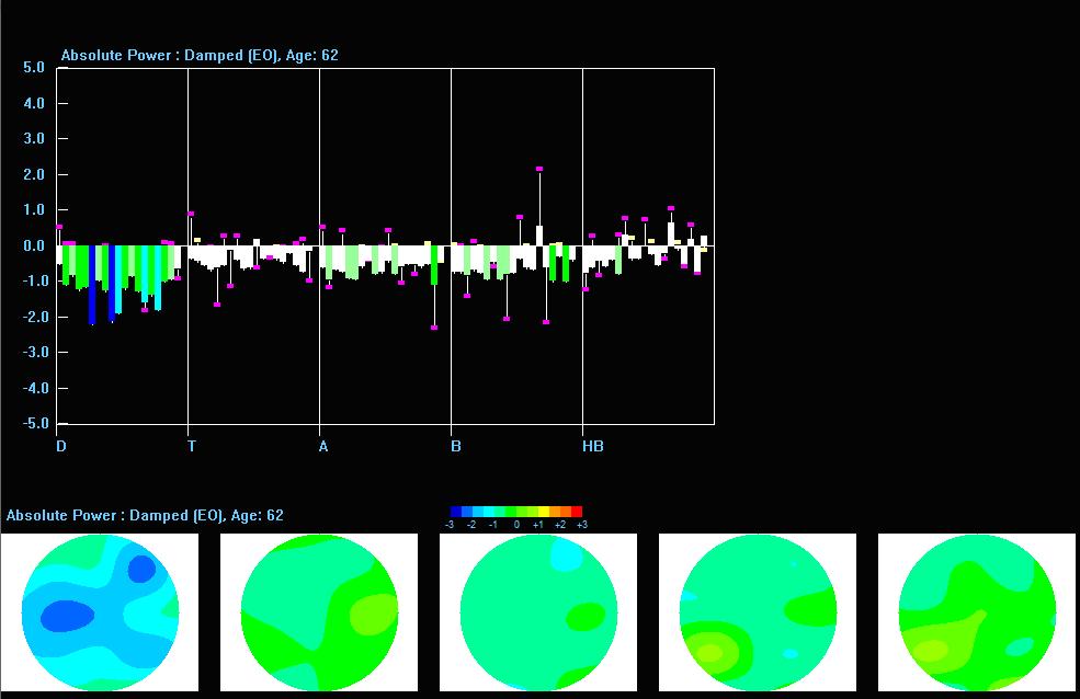

Caption: Z-PLUS LZT Live Z-Score Training with Z-Bars and Z-Maps Display

The client’s EEG values were compared to these values, and differences were displayed in standard deviations. The goal was to train toward z-zero standard deviations.

Caption: Tom Collura

Subsequent advances resulted in 19-channel, real-time surface z-score training and then 19-channel LORETA z-score training, using the LORETA source localization method to train in 3 dimensions. Collura and his colleagues ultimately shifted to the E. Roy John database, BrainDX. Then, they shifted again to a database known as qEEGPro, which was developed using client EEG recordings cleaned of clinical EEG patterns identified by a client questionnaire (qEEG.pro/database/). This approach is based upon questionable assumptions, and many qEEG researchers consulted about this expressed skepticism regarding this database approach (personal communication, John Anderson, 2019-2021).

Caption: qEEGPro 19-Channel sLORETA Z-Score Training

Robert Thatcher and his team continued to work with the Neuroguide database and have continued to develop the features of 19-channel z-score training, most recently with the development of swLORETA, a more precise and accurate iteration of the LORETA source localization method.

Caption: NeuroNavigator swLORETA

This has resulted in a large base of clinicians using this approach. More than 50 publications have presented evidence of the efficacy of z-score neurofeedback training, suggesting widespread acceptance within the scientific literature (https://www.appliedneuroscience.com/PDFs/Z_Score_NFB_Publications.pdf).

Clinical Database Development

Concurrently with the development of the normative database came another approach to protocol development. Skilled and experienced practitioners who also trained new neurofeedback clinicians began to develop what came to be known as a clinical database.

This approach was based on the clinician’s personal experience with often hundreds of clients and their perception of the similarities and differences in the findings associated with those clients. These individuals also consulted the published electroencephalography and neurofeedback research and identified correlations between that information and their experiences.

This led to several semi-automated approaches to assessment and training.

In his article in NeuroConnections (Swingle, 2014), Paul Swingle stated, “For Clinicians, the most accurate databases are clearly clinical.” He describes several logical problems with using normative databases, such as the issue of using a group of supposedly "normal" individuals as a reference standard with which to compare a client with clinical symptoms.

Caption: Paul Swingle

Swingle questioned the fundamental premise of symptom-free individuals selected for a normative database having no underlying abnormalities. He offers the example of heritable disorders such as migraine, schizophrenia, and others, which may have verifiable neurophysiological components that have not manifested due to a lack of triggering factors. In other words, genetic characteristics or predispositions that have not been expressed in the form of identifiable symptoms.

This would lead to a database of individuals who pass all the screening tests yet have notable EEG findings that will become components of the normal standard. Because of this, Swingle suggests that such comparisons are not useful for accurate client assessment and training.

Others also have called into question the concept of the normal individual and pointed out that a symptom-free individual may still have abnormal findings on a clinical EEG assessment strictly based on visual inspection of the EEG by a skilled electroencephalographer (Johnstone & Gunkelman, 2008). They also stated that a database comparison identifies differences from average, not from optimal. The term, normal, is difficult to define, particularly regarding a highly variable measure like the EEG.

Proponents of clinical databases claim exceptional accuracy when used with clinical populations because they were developed from experience with similar individuals experiencing similar symptoms, causal factors, symptom progression, and treatment histories from the general medical and psychiatric communities and psychotherapeutic clinicians.

Because of this reported accuracy and the clinical database’s close alignment with client symptomology, they are often more descriptive and, some say, user-friendly. This is one of the concerns regarding the use of a normative database.

A normative database analysis may produce 200-300 pages of tables, graphs, and topographic brain maps like the ones below. This impressive array of information can be quite overwhelming and difficult to interpret. Questions arise regarding which components of the analysis are important, which relate to the client’s symptoms, and which are useful metrics for planning client training sessions.

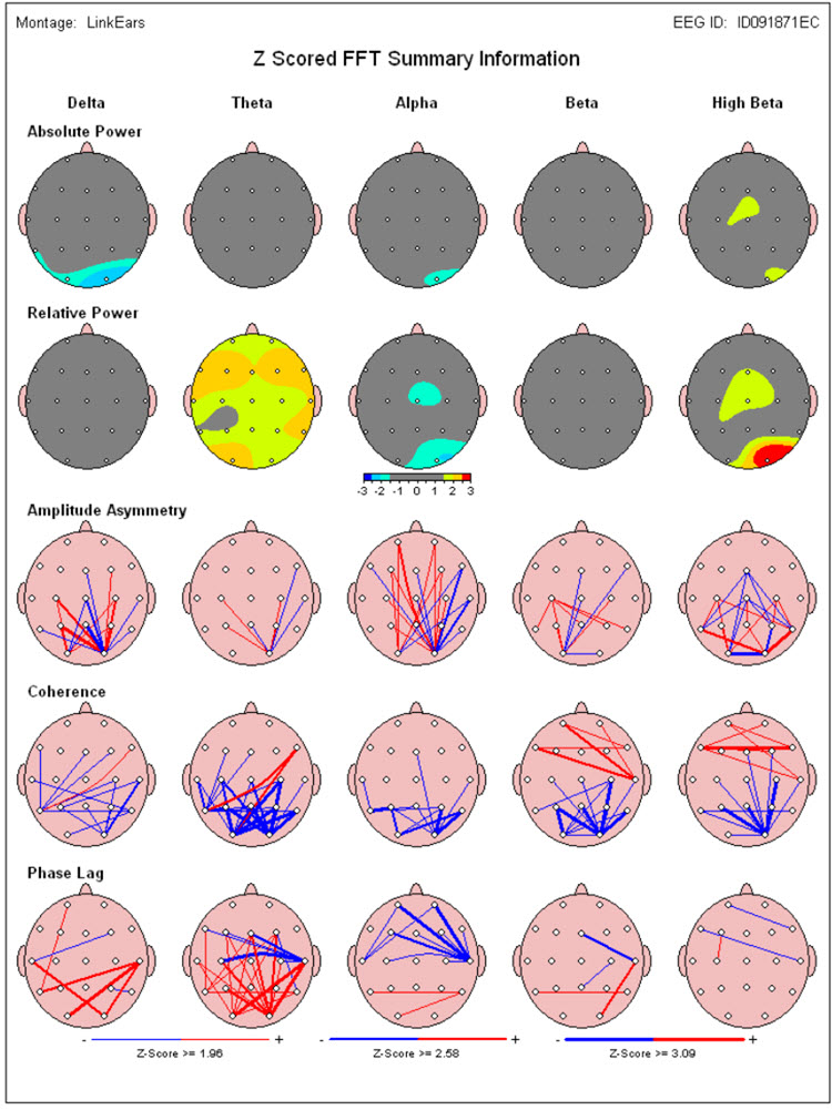
Caption: Image from NeuroGuide Normative Database, Applied Neuroscience.

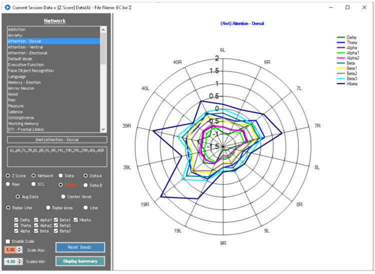
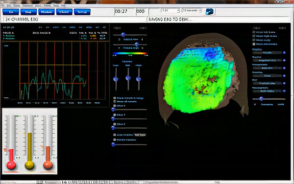
Caption: Image from LORETA Progress Report by Phil Jones.

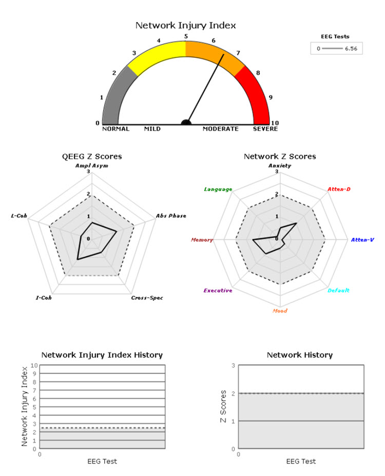
Caption: Image from NeuroGuide Normative Database, Applied Neuroscience.

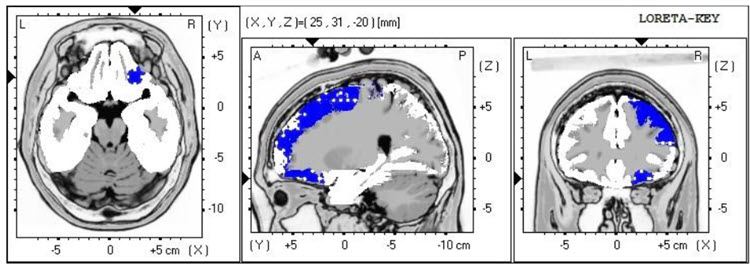
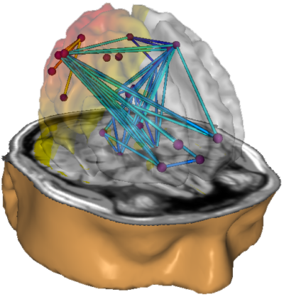
Image from Low Resolution Electromagnetic Tomography (LORETA), Roberto Pascual-Marqui.

Caption: Image from NeuroGuide Normative Database, Applied Neuroscience.

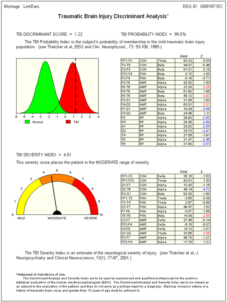
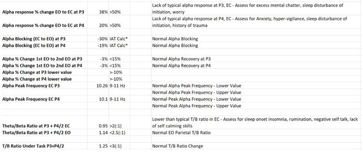
On the other hand, a clinical database is often more descriptive. Some only provide graphs and tables, but most also suggest relationships between the findings and probable client symptoms. Swingle’s Clinical Q provides a data analysis that shows differences from expected data and offers "probes" for client symptoms or behaviors that may be consistent with these findings.

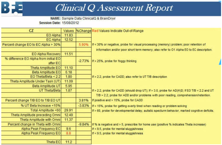
Caption: Clinical Q example report.

Peter Van Deusen

One of the earliest clinical databases was created by Peter Van Deusen (Ribas et al., 2016), who initially studied with Joel Lubar. He aimed to identify client symptoms and behavioral issues without utilizing diagnostic categories so that clients could be trained using neurofeedback approaches no matter what the issue.

The culmination of his years of work with clients, training practitioners, and studying the EEG was an approach known as The Learning Curve (TLC). TLC organized client symptoms and findings into six broad categories and identified training approaches to train these clients.

Caption: Peter Van Deusen.

Richard Soutar

Another approach to this method, and arguably the most comprehensive, is the New Mind Maps developed by Richard Soutar. This system has a variety of levels of analysis up to 19 channels and a detailed report that covers most of the typical metrics and provides narrative content and protocol recommendations for standard amplitude training and z-score training. It offers advice about additional interventions such as audio-visual entrainment (AVE).

Caption: Richard Soutar

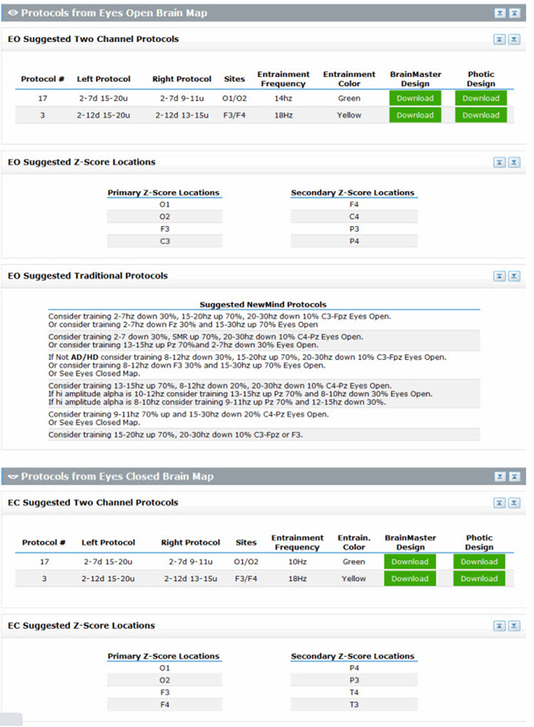
Caption: New Mind Maps, Richard Soutar – http:/www.newmindmaps.com.

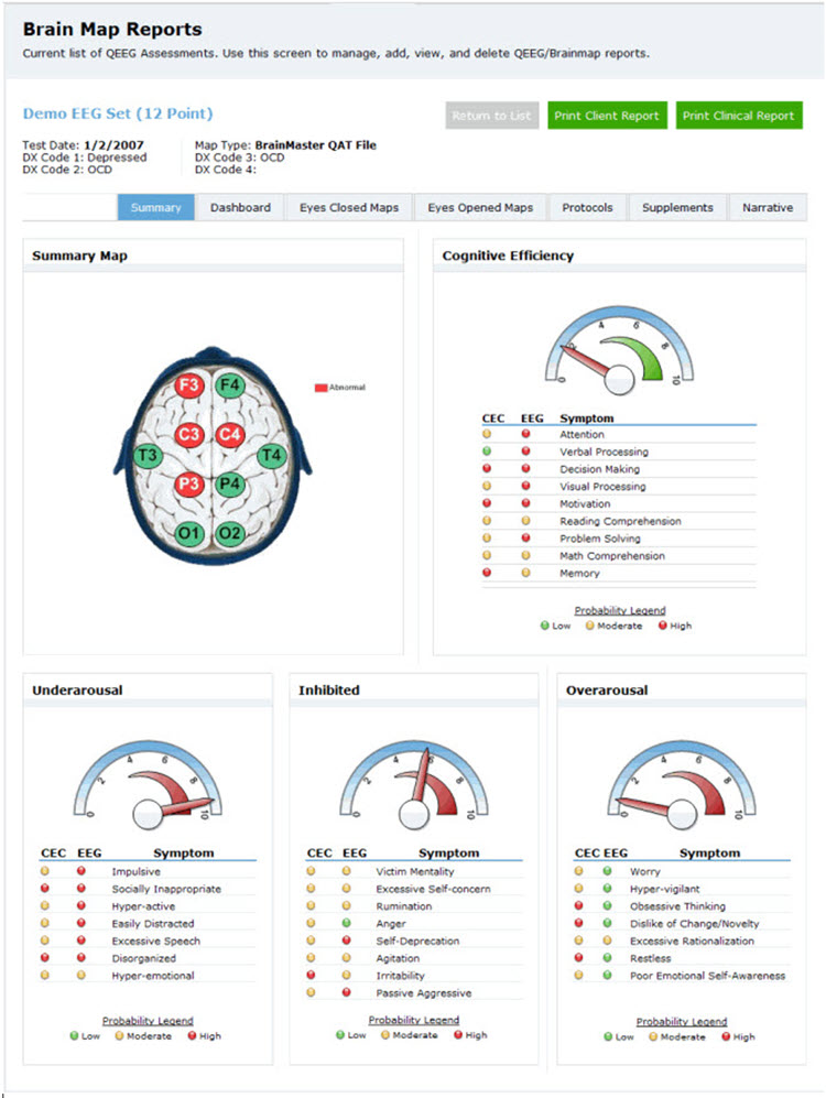
Caption: New Mind Maps, Richard Soutar – http:/www.newmindmaps.com.

John Demos

The Jewel Clinical Database, developed by John Demos, author of Getting Started with Neurofeedback (2nd ed.), is another clinical database for ages 7-19 and adults that produces surface and sLORETA representations (maps, graphs, etc.) and training recommendations based on client checklists.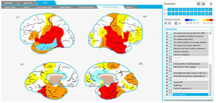

Caption: The Jewel Clinical Datavase, John Demos.

Caption: John Demos.

John Anderson

John Anderson developed an assessment for the Nexus/BioTrace system known as the NewQ.

Caption: John Anderson

This system is like the Clinical Q of Paul Swingle and uses 6 locations, recorded sequentially, two locations at a time. There are four age ranges: 6-11, 12-15, 16-20, and 21+ (adult).

Caption: NewQ, John Anderson.

The following is the disclaimer from the NewQ assessment. These cautions are worth keeping in mind when utilizing such an approach to assessment.

Disclaimer: This assessment tool is based upon a general understanding of the EEG literature plus the author's clinical experience. It should not be viewed as a statistically validated or rigorously referenced instrument and constitutes a set of clinical observations. It is not a diagnostic instrument, and results must be evaluated based on the client's presenting concerns. The clinical judgment of the practitioner must remain primary in any assessment process.

The clinical database approach is valuable in providing practitioners with a perspective on client assessment based on the author’s knowledge and experience. It can be a helpful shortcut for beginning practitioners and experienced clinicians as they benefit from different clinical perspectives.

However, because the sensor locations are often recorded sequentially (except for Soutar’s 19-channel version of New Mind Maps), the assessments cannot calculate such important metrics as phase and coherence, except for sensor locations recorded simultaneously. Also, the perspective of the designer/author is quite subjective and, while reflecting knowledge and experience, may also reflect unconscious biases and assumptions that are not rigorously grounded in published research.

Ideally, there will eventually be a blending of the normative database approach with the clinical assessment to the point where a truly accurate and effective "expert" system can be designed to develop best practices for neurofeedback training.

A Guide to Interpreting qEEG Topographic Maps

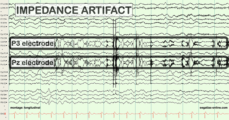
Reading topographic maps of the EEG may seem straightforward and relatively simple. Z-score maps highlight areas that deviate from typical values compared to normative databases adjusted for age and sometimes gender and handedness. When an area on the map shows excessive activity in a particular EEG frequency, targeted sensor placement and effective client training can help normalize these levels. Conversely, reduced activity in an area may result in efforts to enhance it.

However, the reality is more complex. EEG recordings often exhibit significant artifacts from multiple sources, such as environmental interference (e.g., 50- or 60-Hz electrical noise) and physiological factors like eye blinks, movements, heartbeats, and muscle contractions. We must clean EEG data to ensure its integrity. This requires distinguishing between genuine EEG activity and transient phenomena such as drowsiness, sleep, or normal variants that do not signify pathology. While important for an accurate EEG report, these EEG features should not factor into statistical analyses.

Creating topographic EEG maps should be considered one of the last stages of a clinical assessment, not its primary focus.

Therefore, adhering to a careful progression from data collection to comprehensive analysis is essential instead of relying on automated artifact rejection algorithms and immediately generating maps.

Focusing neurofeedback training on areas associated with problematic symptoms is important for effective intervention. Simply targeting any abnormality detected in the EEG may not address the underlying issues and could lead to unintended consequences.

Atypical EEG findings can arise from various factors, including exceptional skills, compensatory changes due to illness or injury, developmental differences, or unique characteristics that do not necessarily indicate pathology. Therefore, careful clinical assessment and interpretation are necessary to determine whether observed deviations require correction.

By focusing on symptom-based training associated with understanding the clinical picture, clinicians can ensure that neurofeedback protocols address specific concerns and optimize outcomes for individuals undergoing training.

The following is an example of an EEG recording of a 76-year-old male with complaints of "brain fog," memory problems, lack of energy, slow cognitive processing, and difficulty sleeping.

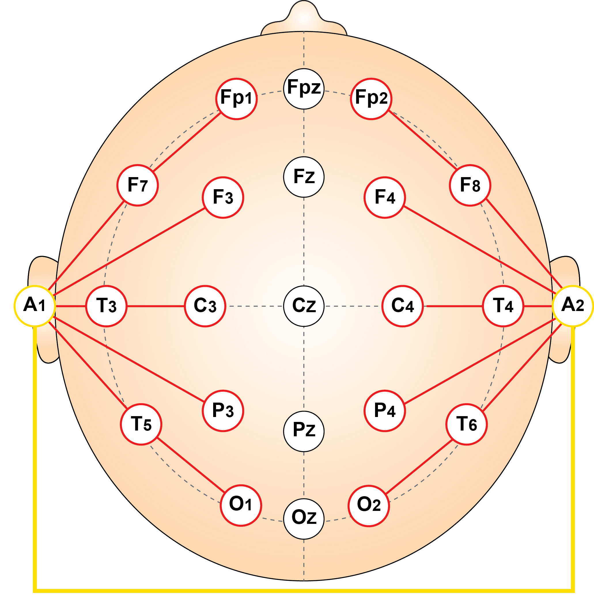
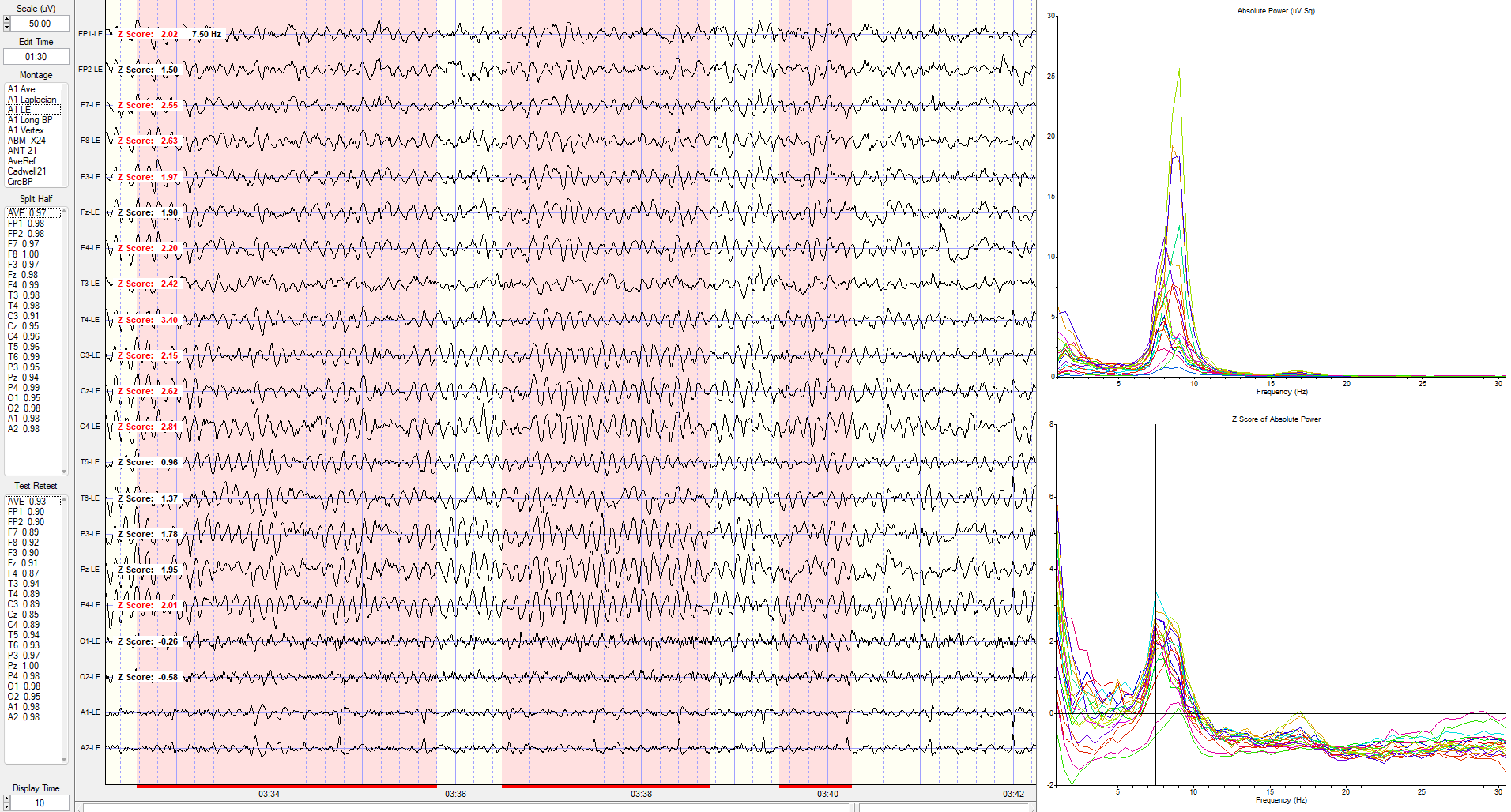
Eyes-Closed Linked Ears (ECLE) Montage

This is a 50-uV scale, 10-sec display. Note the persistent ECG artifact in multiple channels, most clearly seen in reference channels (red outline at the bottom). The peak alpha frequency is approximately 8 Hz, the amplitude is 12-25 uV at the parietal sensors, and there is a small electrode pop in the F4 sensor (blue outline in this and subsequent montages).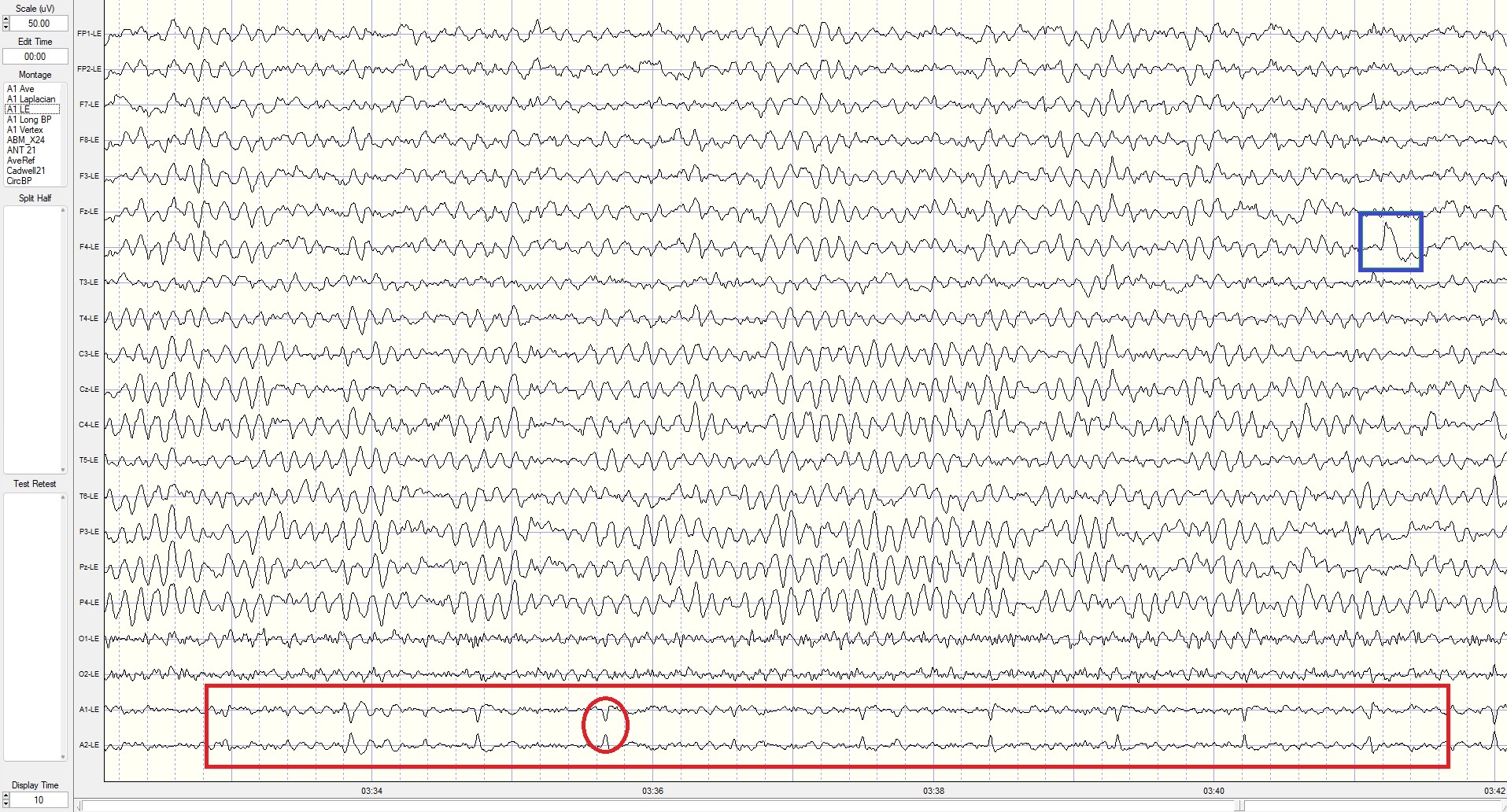

Eyes-Closed Longitudinal Bipolar (ECLBP) Montage

This is a 50-uV scale, 10-second display. The alpha frequency is 8 Hz, and the amplitude is 10-30 uV in parietal-occipital derivations. Note that the rhythmic activity (frontal alpha) seen in the linked ears montage is not present in prefrontal–frontal derivations in this bipolar montage, indicating it was the result of reference contamination in the previous montage.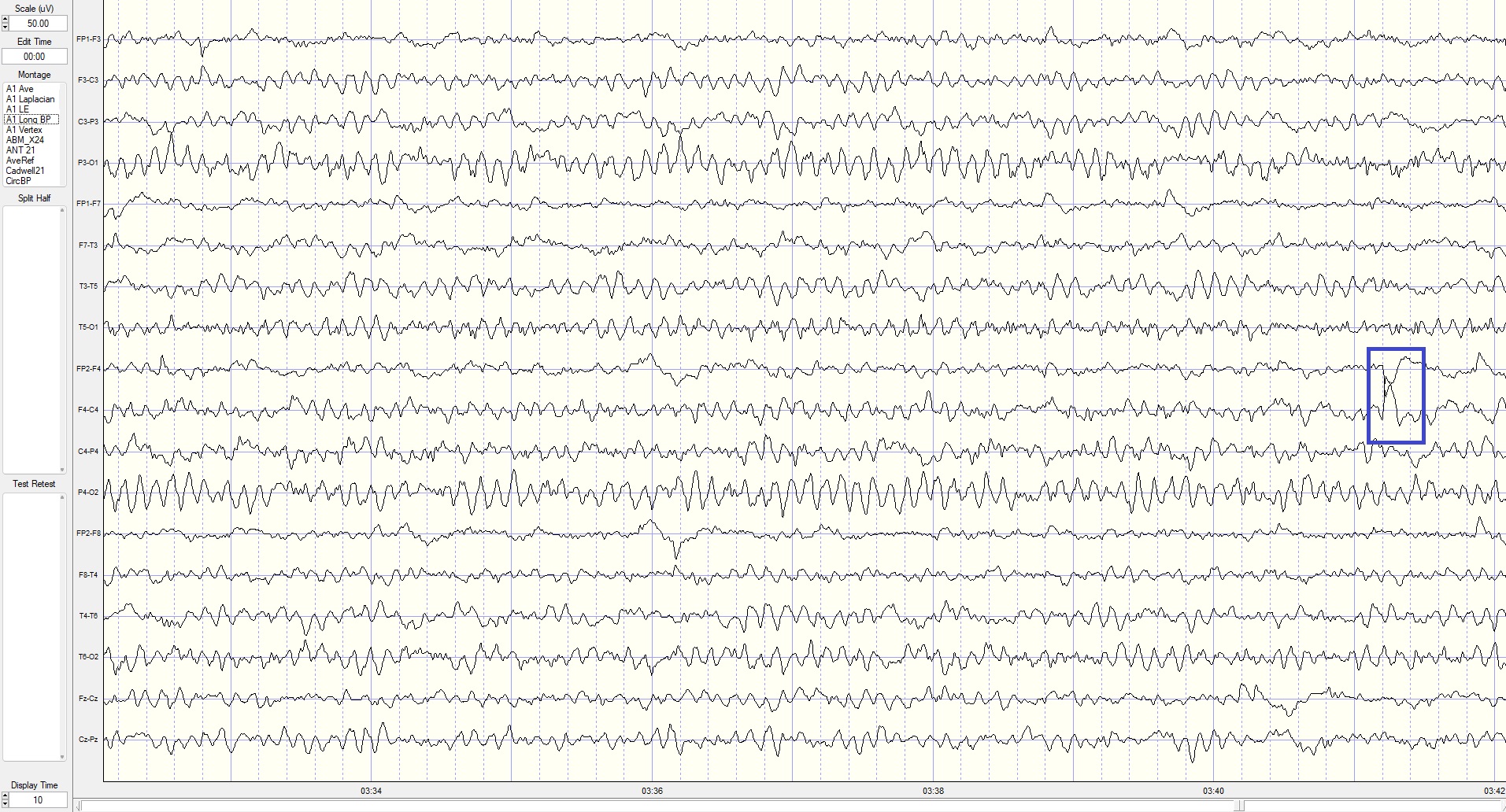

Eyes-Closed Average Reference (ECAVE) Montage

This is a 50-uV scale, 10-second display. The alpha frequency is 8-9 Hz, and the amplitude is 5-15 uV at the occipital and 10-18 uV at the parietal sensors. Note the delta activity at the parietal sensors (green outline) and EMG artifact at the occipital sensors.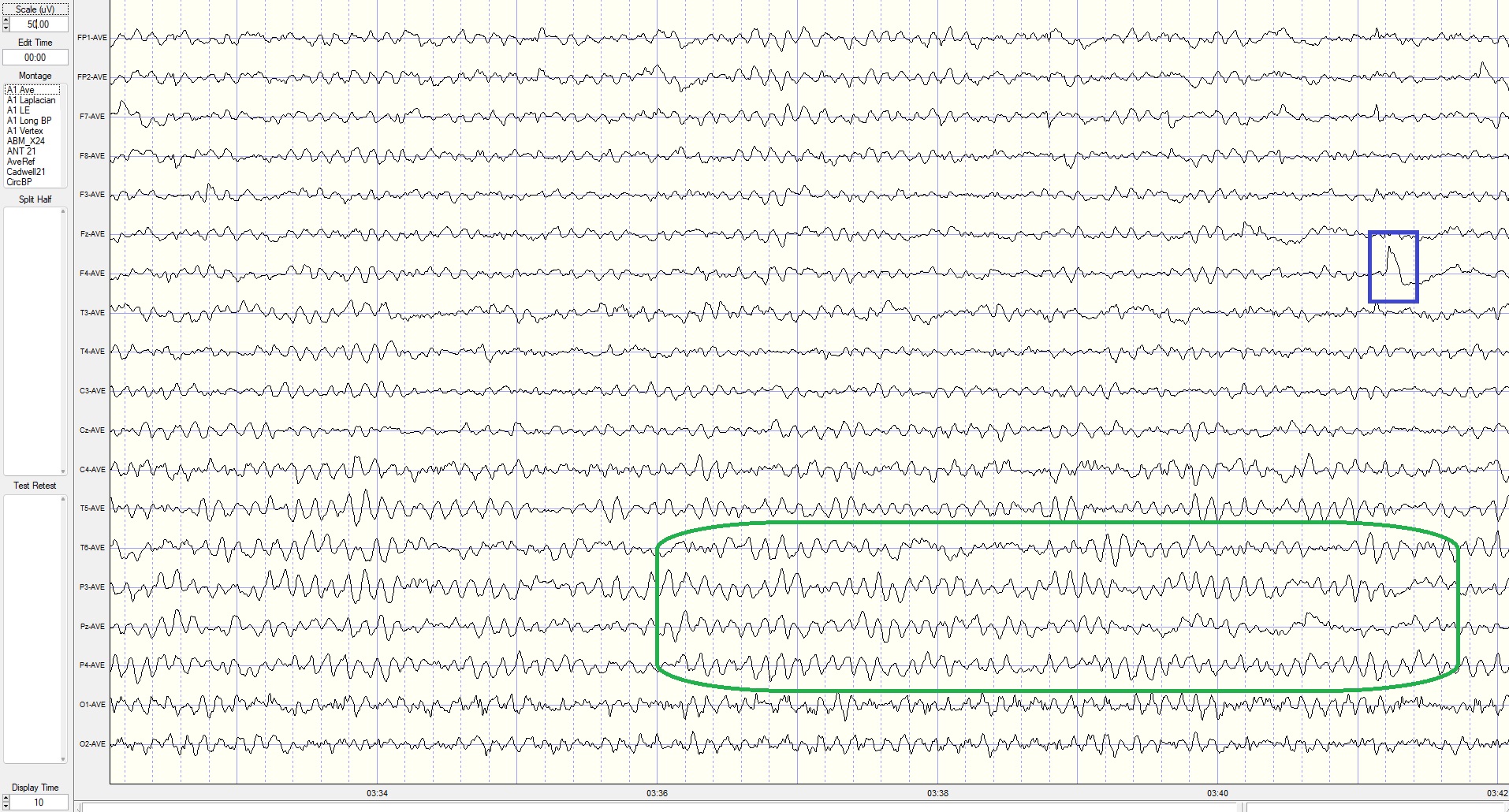

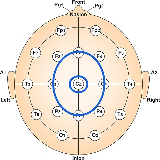
Eyes-Closed Laplacian (ECLP) Montage

This is a 400-microampere (uA) scale, 10-second display. The alpha frequency is 8-9 Hz, with the highest current density in parietal sensors. EMG artifact continues in occipital sensors, and delta is more pronounced in the parietal area. Electrode pop in F4 sensor. The lack of prefrontal and frontal alpha activity suggests reference contamination in the linked ears montage above.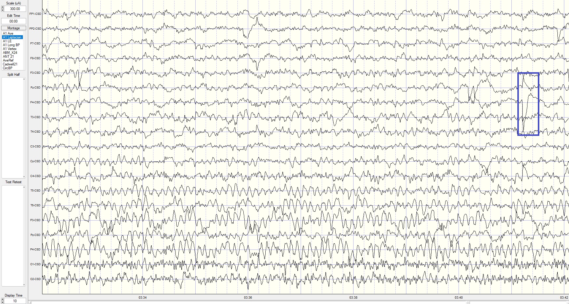

Eyes-Closed Linked Ears (ECLE) Montage

A linked ears montage in NeuroGuide with FFT absolute power spectral display at the top right with a line indicating the highest amplitude at 9 Hz is at the P4 electrode.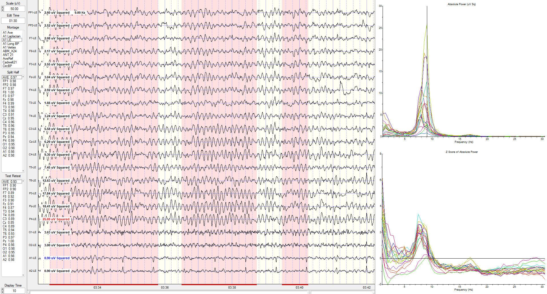




The same image showing the maximum power at 8 Hz is at the C4 electrode.





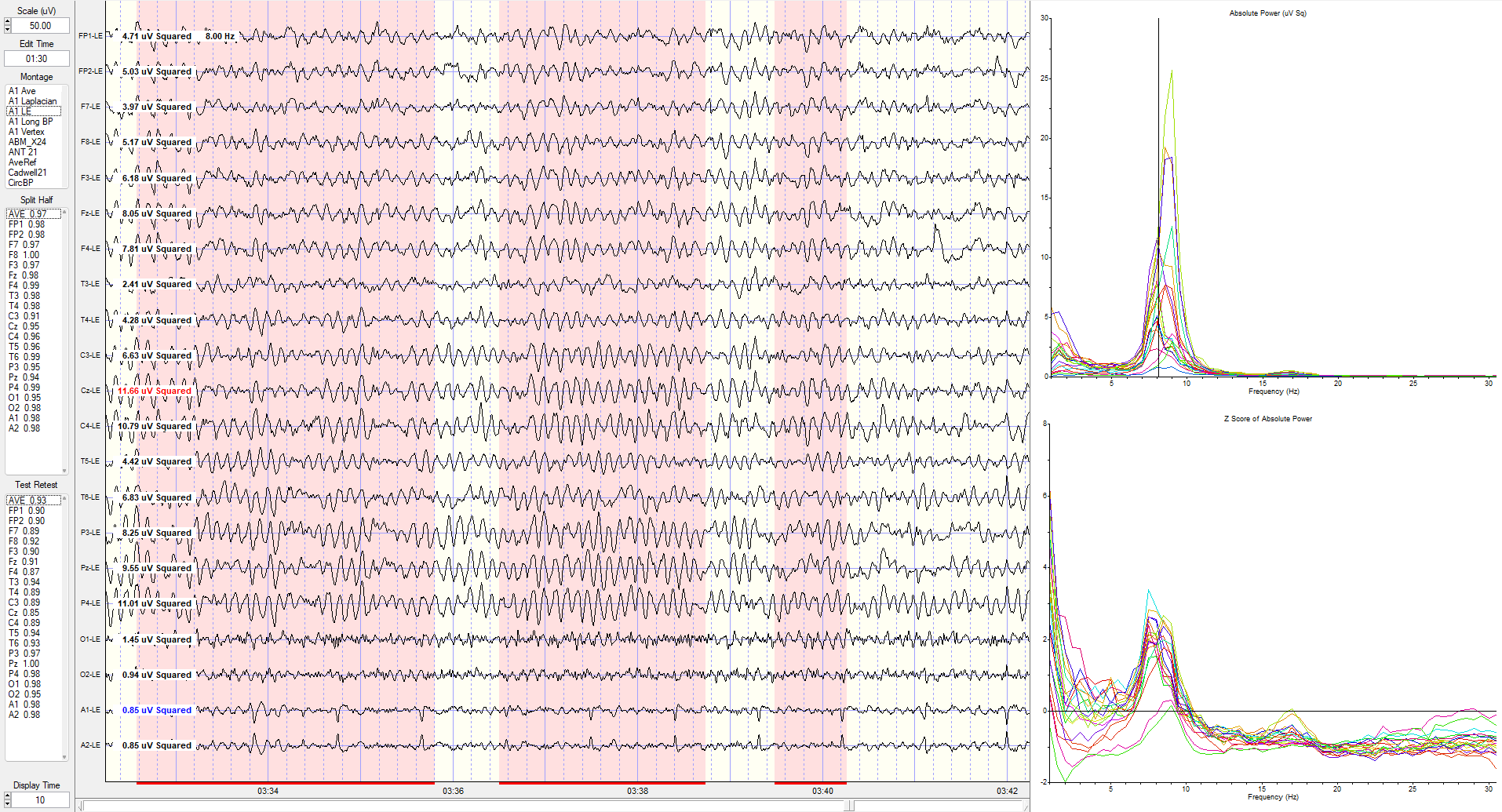
The same linked ears montage image shows the peak activity at 7.5 Hz, which is generally 1-3 SD greater than typical values at multiple locations (see z-score indicators on the left side of tracings next to electrode location labels).

Eyes-Closed Longitudinal Bipolar (ECLBP) Montage

This spectral display shows a longitudinal bipolar montage indicating the maximum z-scores at 2.5 Hz.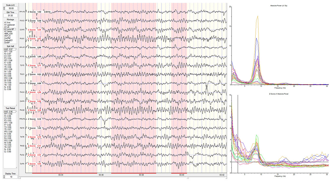






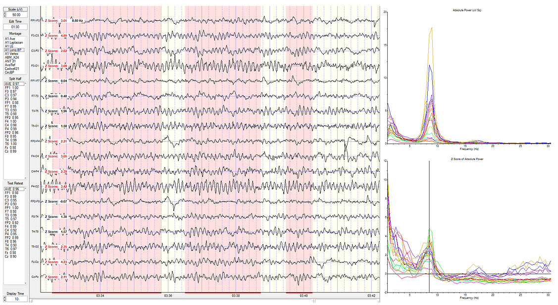
Eyes-closed longitudinal bipolar montage showing standard deviations at 8.5 Hz.

Eyes-Closed Average Reference (ECAVE) Montage

Average reference montage showing deviations at 2.5 Hz.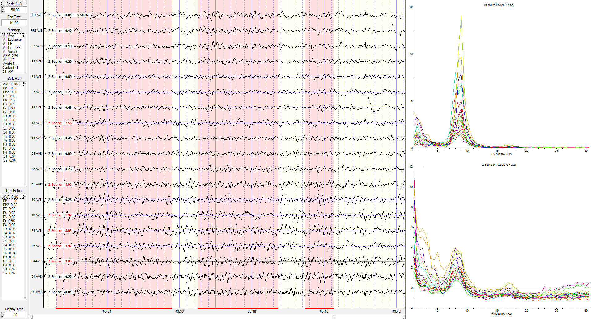

Eyes-Closed Laplacian (ECLP) Montage

Laplacian montage showing current source density (CSD) z-scores at 3 Hz.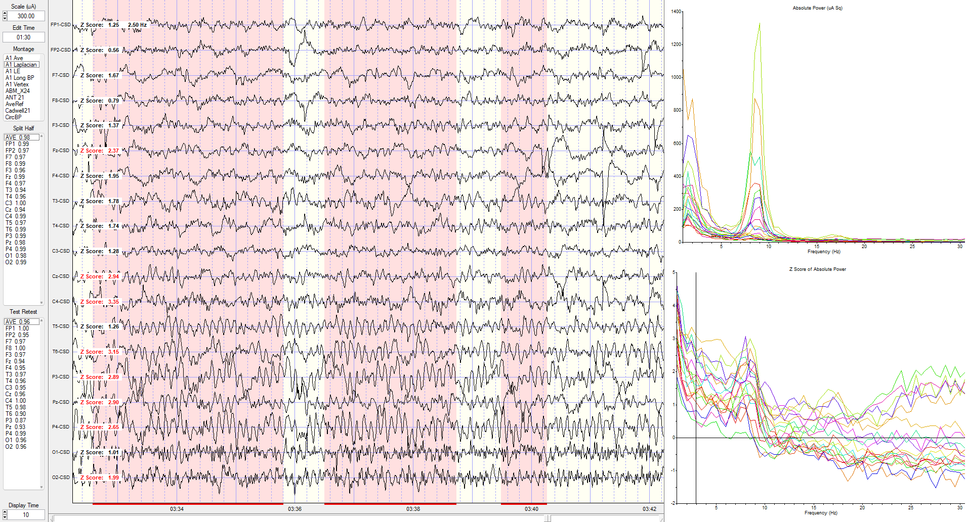

Eyes-Closed Linked Ears (ECLE) Montage

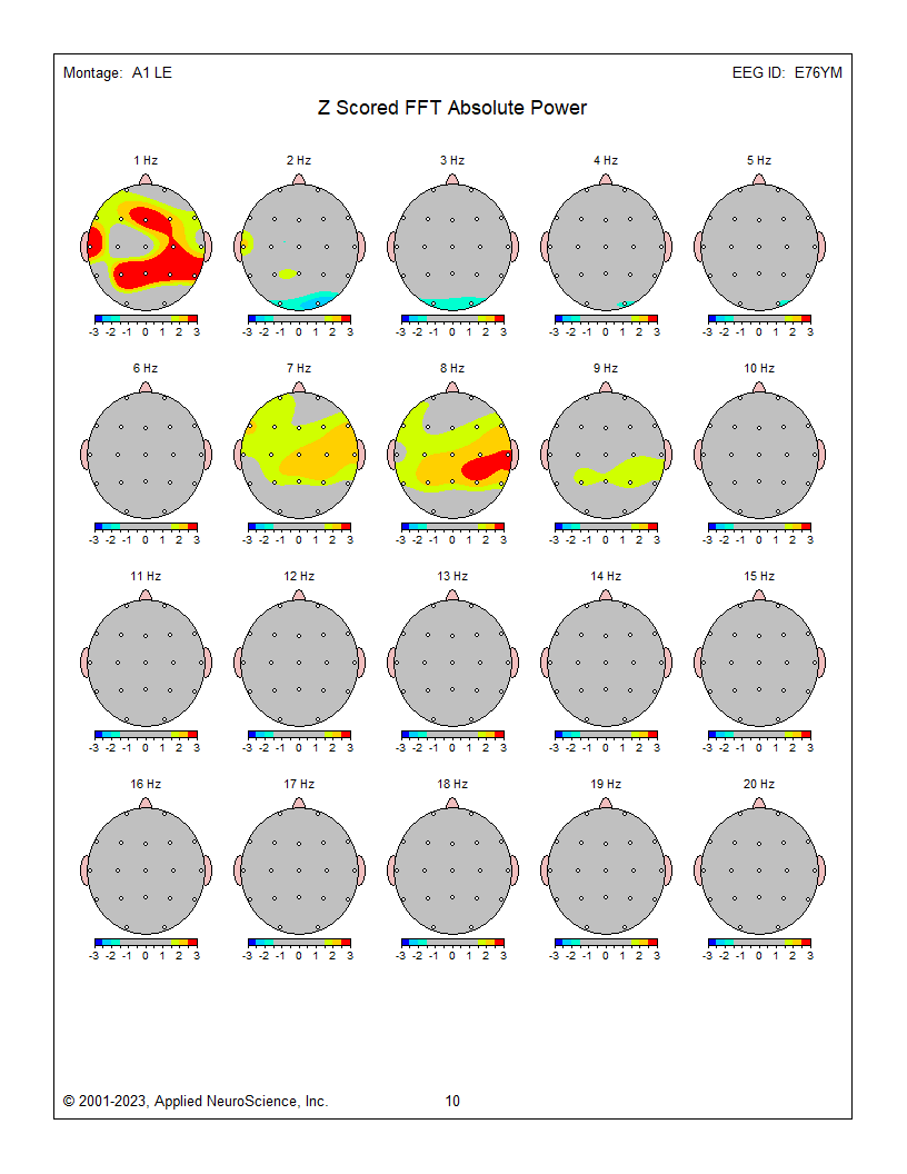
These absolute power topographic maps represent 1 minute and 30 seconds of a recording from an eyes-closed linked ears montage. Each small head map represents a virtual view of the top of the head with the nose at the top. The absolute power (microvolts squared) values correspond to the colored scale below each map. Red represents the greatest value, and blue is the lowest value for each 1 Hz frequency bin. The P4 electrode shows a power value of 36 in the 9 Hz frequency bin. Each bin has its own scale.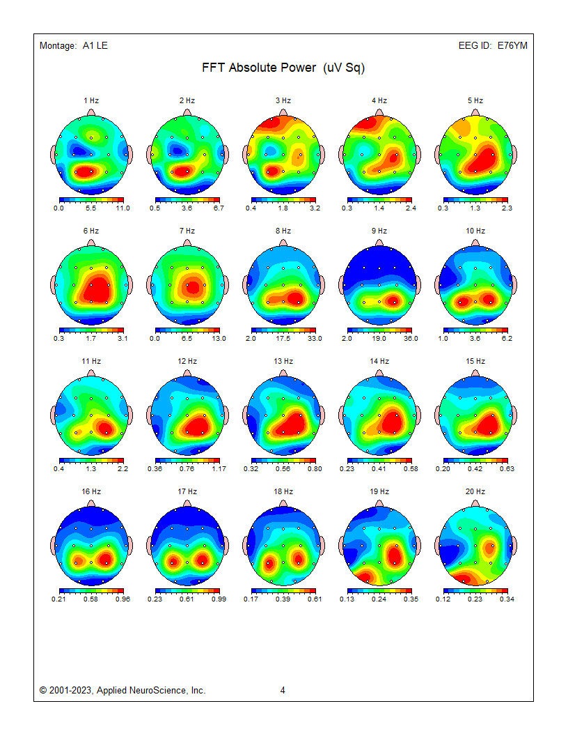

Z-Score Absolute Power

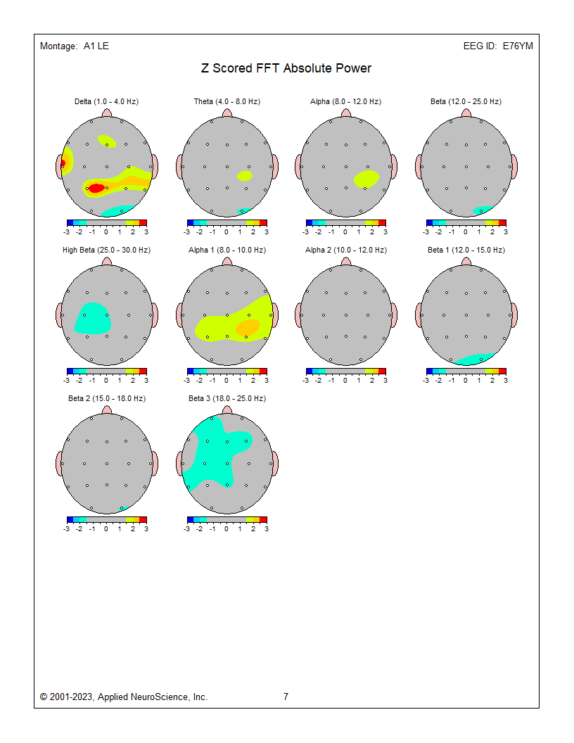
1-Hz frequency bin maps showing maximum to minimum deviations compared to the NeuroGuide normative database for a linked ears montage. The scale is from -3 (blue) to +3 (red) standard deviations (SD). The excess activity at 1 Hz is likely due to the ECG artifact noted earlier. The heart beats at about 1 beat per second, which equals 1 Hz. Excess activity is seen at 7-9 Hz.

Frequency band maps (like delta, theta, alpha, and beta) show the entire frequency band and lack the resolution of the individual 1-Hz frequency bin maps. The delta map generally shows excess delta activity, which misidentifies the ECG artifact that was seen at 1 Hz in the frequency bin maps and the visual inspection of the EEG.



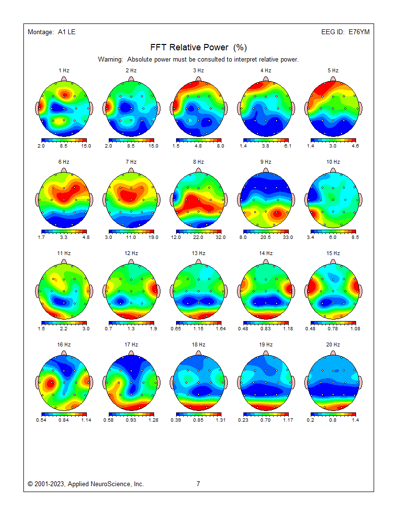
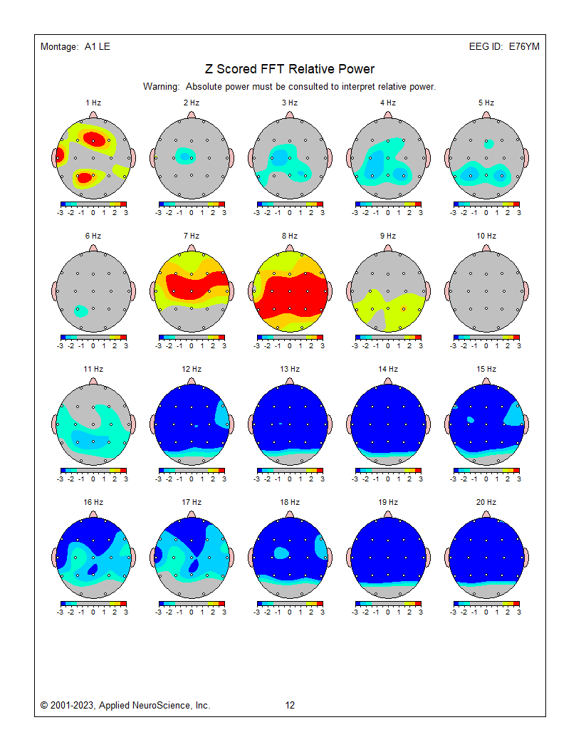
These are relative power topographic maps representing 1 minute and 30 seconds of data from an eyes-closed linked ears montage. They show relative power values (percentages) that compare the value in each 1 Hz bin to the broadband EEG (0.5 – 30 Hz). This information is displayed as a colored scale below each map, with red representing the highest percentage and blue representing the lowest percentage for each 1-Hz frequency bin. Note that 9 Hz contains 33 percent of the total EEG power at the P4 electrode location. Each head map has its own scale.


These are z-score relative power 1-Hz frequency bin maps showing maximum to minimum deviations compared to the NeuroGuide normative database using a linked ears montage. The scale is from -3 (blue) to +3 (red) standard deviations (SD). Note that this page represents relative power, showing the relative value of each 1 Hz bin compared to the EEG as a whole. This can result in areas showing incorrect abnormal z-score values at some frequencies because other frequencies are abnormal in the opposite direction. For example, frontal, central, and parietal activity at 8 Hz is excessive in the image below, causing apparent deficient activity in the same areas at multiple frequencies because 8 Hz takes up too much of the percentage "pie."

The previous examples show the progression of EEG analysis from viewing the recorded EEG through spectral analysis to topographic maps representing absolute and relative power and z-score maps showing deviations from expected values when client results are compared to a normative database.

The raw tracings and the spectral displays show examples from multiple montages (sensor comparisons) and help to highlight that what is seen is highly dependent upon which comparisons are used. So far, The topographic map examples have all used the linked ears montage and only showed one perspective on the EEG results. Now, we will look at the same data presented as topographic maps using different montages.

Eyes-Closed - 3 Montages

Eyes-closed average montage absolute power topographic map for 1-20 Hz, eyes-closed linked ears absolute power topographic map for 1-20 Hz, and eyes-closed Laplacian absolute power topographic map for 1-20 Hz.


Eyes-closed average z-score absolute power topographic map for 1-20 Hz, eyes-closed linked ears z-score absolute power topographic map for 1-20 Hz, and eyes-closed Laplacian montage z-score absolute power topographic map for 1-20 Hz. Notice the differences between the average, Laplacian, and linked ears reference maps. Which one should we follow when completing our assessment?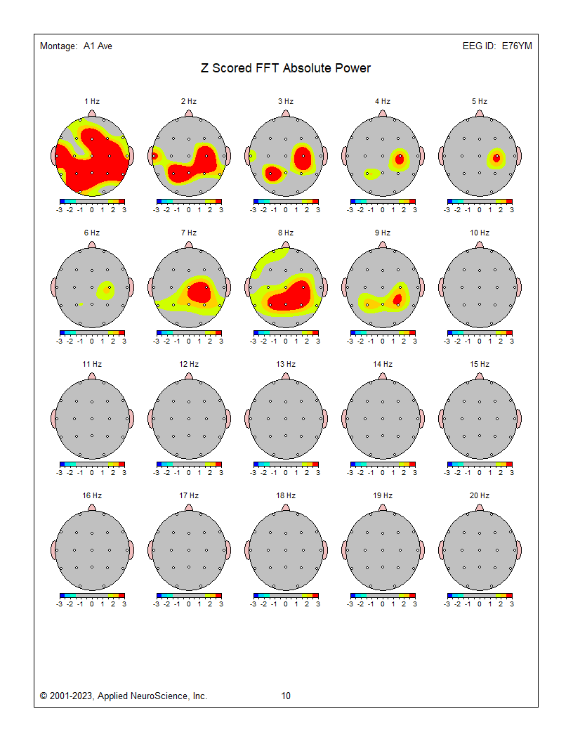



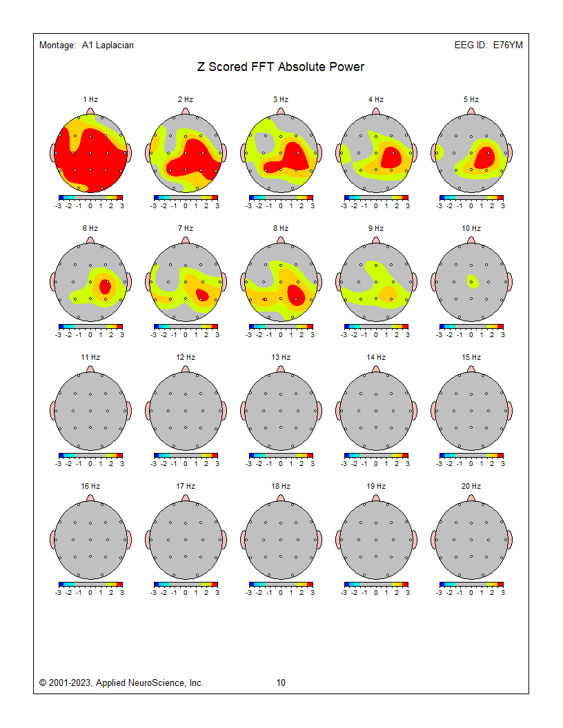
The average reference and Laplacian montages show fairly similar results and correspond to some of the other indicators and may generally represent the client’s presenting issues of brain fog, memory issues, and slow cognitive processing.

Several posts and Neurofeedback Tutor have addressed the issue of montage selection. Nunez and Srinivasan's (2006) Electrical Fields of the Brain (2nd ed.) is an excellent resource for more in-depth information.

For this example, we are confronted with significant differences between the linked ears results and average reference and Laplacian montage results, when there is excess activity in the 2-6 Hz range of delta and theta.

The Laplacian montage uses an average of the current flow from electrodes immediately surrounding the electrode of interest as a localized average reference using current rather than voltage as its metric. This has been described as more accurate in identifying local activity while minimizing general effects such as those from medication, drowsiness, and others. This can help highlight local abnormalities, which can be lost or masked by other montages.

The average reference montage uses an average of all scalp electrodes to serve as the reference for each electrode, thus eliminating the ear or mastoid reference. This helps remove contributions from these reference electrodes, common to all electrode pairings when using the linked ears or linked mastoid reference montage.

Each of these montage choices has benefits and limitations. The benefits have been mentioned above, but what are the limitations? The average reference montage, like all montages, is subject to the differential amplifier's common mode rejection phenomenon. Sources (electrical activity such as EEG, ECG, EMG, EOG, EMF) that are the same in frequency and, to a lesser extent, in amplitude are rejected, while sources that are different are retained. If multiple sources (electrode locations) of delta activity contribute to the average, and this average is then compared to a location that does not show delta activity, then there is a difference between the signals. That difference is retained and displayed in the topographic maps and, of course, in the EEG tracings, resulting in apparently abnormal delta activity where it does not exist. The same is true of the linked ears/mastoid reference and, to a lesser extent, of the Laplacian montage.

Therefore, we look for agreement among multiple montages, being particularly attentive to the various bipolar montages that allow revealing comparisons when viewing the EEG tracings.

In the present example, though earlier we mentioned that the delta activity was confined to the 1 Hz effect from the ECG (heartbeat) artifact, we can see from the Laplacian and average montages that there is substantial agreement on a broader frequency distribution of delta/theta activity that exceeds statistical significance. Thus, the recommendation is to begin training by focusing on these excesses.

Glossary

bins: frequency ranges, which may be as narrow as 1 Hz, into which the EEG power spectrum is divided.

Eyes-Closed Average Reference (ECAVE) montage: a method of EEG electrode montage where the average of all EEG channels is subtracted from each individual channel's EEG signal. This technique is often used to remove common noise sources and enhance the signal-to-noise ratio, particularly during eyes-closed conditions when the brain is relatively more relaxed.

Eyes-Closed Laplacian (ECLP) montage: a spatial filtering technique in qEEG where the Laplacian transform is applied to the EEG signal recorded during eyes-closed conditions. This transform emphasizes local changes in EEG activity while reducing the influence of distant sources, thus enhancing spatial resolution.

Eyes-Closed Linked Ears (ECLE) montage: referencing the EEG signal recorded during eyes-closed conditions to an electrode placed on each earlobe, with the two ear electrodes linked together. This montage is used to minimize common noise sources and provide a stable reference for EEG analysis.

Eyes-Closed Longitudinal Bipolar (ECLBP) montage: a bipolar referencing method in qEEG where each EEG channel is computed as the difference between neighboring electrodes. This montage is often applied during eyes-closed conditions to enhance the detection of local variations in EEG activity.

montage: EEG recording configuration that groups electrodes (combines derivations) to monitor EEG activity.

z-score absolute power: a statistical measure used in qEEG analysis to quantify the deviation of absolute power values within specific frequency bands from a normative database. It indicates how many standard deviations a particular absolute power measurement is from the mean of the reference population, providing a measure of relative EEG activity levels across different frequency bands.

Test Yourself

Customers enrolled on the ClassMarker platform should click on its logo to take 10-question tests over this unit (no exam password).

REVIEW FLASHCARDS ON QUIZLET

Click on the Quizlet logo to review our chapter flashcards.

Visit the BioSource Software Website

BioSource Software offers Physiological Psychology, which satisfies BCIA's Physiological Psychology requirement, and Neurofeedback100, which provides extensive multiple-choice testing over the Biofeedback Blueprint.

Assignment

Now that you have completed this unit, explain the rationale for z-score training using a normative database.

References

Ayers, M. E. (1977). EEG Neurofeedback to bring individuals out of Level Two Coma [Abstract]. Biofeedback and Self-Regulation, 20(3), 304–305.

Berger, H (1929). Über das elektroenkephalogramm des menschen. Arch Psychiatr Nervenkr 87(1), 527–570.

Budzynski, T. H. (1977). Tuning in on the twilight zone. Psychology Today, 11, 38–44.

Budzynski, T. H. (1996). Brain brightening: Can neurofeedback improve cognitive process? Biofeedback, 24, 14–17.

Byers, A. P. (1998). Neurotherapy reference library (2nd ed.). Applied Psychophysiology and Biofeedback.

Evans, J. R., Dellinger, M. B., & Russell, H. L. (Eds.) (2020). Neurofeedback: The first fifty years. Academic Press.

Fehmi, L. G., & Robbins, J. (2008). Sweet surrender-Discovering the benefits of synchronous alpha brainwaves (pp. 231-254). Measuring the immeasurable: The scientific case for spirituality. Sounds True, Inc.

Fein, G., Galin, D., Johnstone, J., Yingling, C. D., Marcus, M., & Kiersch, M. E. (1983).EEG power spectra in normal and dyslexic children. I. Reliability during passive conditions. Electroencephalogr Clin Neurophysiol, 55(4), 399-405. https://doi.org/10.1016/0013-4694(83)90127-x

Hardt, J. V., & Kamiya, J. (1978). Anxiety change through electroencephalographic alpha feedback seen only in high anxiety subjects. Science, 201(4350).79-81. https://doi.org/10.1126/science.663641 PMID: 663641.

John, E. R., Ahn, H., & Prichep, L., Trepetin, M., Brown, D., & Kaye, H. (1980). Developmental equations for the electroencephalogram. Science, 210(4475), 1255-1258. https://doi.org/10.1126/science.7434026

Johnstone, J. & Gunkelman, J. (2003). Use of databases in QEEG evaluation. Journal of Neurotherapy, 7, 3-4, 31-52. https://doi.org/10.1300/J184v07n03_02

Kamiya, J. (1968). Conscious control of brain waves. Psychology Today, 1, 56-60.

Legarda, S. B., McMahon, D., Othmer, S., & Othmer S. (2011). Clinical neurofeedback: Case studies, proposed mechanism, and implications for pediatric neurology practice. J Child Neurol., 26(8),1045-1051. https://doi.org/10.1177/0883073811405052

Leong, S. L., Vanneste, S., Lim, J., Smith, M., Manning, P., & De Ridder, D. (2018). A randomised, double-blind, placebo-controlled parallel trial of closed-loop infraslow brain training in food addiction. Sci Rep 8(11659). https://doi.org/10.1038/s41598-018-30181-7

Lubar, J. F., & Bahler, W. W. (1976). Behavioral management of epileptic seizures following EEG biofeedback training of the sensorimotor rhythm. Biofeedback Self Regul, 1(1), 77-104. https://doi.org/10.1007/BF00998692. PMID: 825150.

Lubar, J. F., Shabsin, H. S, Natelson, S. E., Holdson, S. E., Holder, G. S., Whittsett, S. F., Pamplin, W. E., & Krulikowski, D. I. (1981). EEG operant conditioning in intractable epileptics. Archives of Neurology, 38, 700–704.

Lubar, J. F., & Shouse, M. N. (1976). EEG and behavioral changes in a hyperkinetic child concurrent with training of the sensorimotor rhythm (SMR): A preliminary report. Biofeedback Self Regul,1(3), 293-306. https://doi.org/10.1007/BF01001170. PMID: 990355.

Marzbani, H., Marateb, H. R., & Mansourian, M. (2016). Neurofeedback: A comprehensive review on system design, methodology and clinical applications. Basic and clinical neuroscience, 7(2), 143–158.

Monastra, V. J., Lubar, J. F., Linden, M., VanDeusen, P., Green, G., Wing, W., Phillips, A., & Fenger, T. N. (1999). Assessing attention deficit hyperactivity disorder via quantitative electroencephalography: An initial validation study. Neuropsychology, 13(3), 424–433. https://doi.org/10.1037/0894-4105.13.3.424

Nuwer, M. R., & Coutin-Churchman, P. (2014). Brain mapping and quantitative electroencephalogram. Encyclopedia of the Neurological Sciences (2nd ed.). Elsevier.

Oken, B. S., & Chiappa, K. H. (1988). Short-term variability in EEG frequency analysis. Electroencephalogr Clin Neurophysiol, 69, 191–198. https://doi.org/10.1016/0013-4694(88)90128-9

Peniston, E. G., & Kulkosky, P. J. (1989). Alpha-theta brain wave training and beta-endorphin levels in alcoholics. Alcoholism, Clinical and Experimental Research, 13, 271 – 279. https://doi.org/10.1111/J.1530-0277.1989.TB00325.X

Peniston, E. G., & Kulkosky, P. J. (1990). Alcoholic personality and alpha-theta brain wave training. Medical Psychotherapy, 3, 37–55.

Putman, J. A., Othmer, S. F., Othmer, S., & Pollock, V. E. (2005). TOVA results following inter-hemispheric bipolar EEG training. Journal of Neurotherapy: Investigations in Neuromodulation, Neurofeedback and Applied Neuroscience, 9(1), 37-52. https://doi.org/10.1300/J184v09n01_04

Ribas, V. R., Ribas, R., & Martins, H. (2016). The learning curve in neurofeedback of Peter Van Deusen: A review article. Dementia & Neuropsychologia, 10(2), 98–103. https://doi.org/10.1590/S1980-5764-2016DN1002005

Rogala, J., Jurewicz, K., Paluch, K., Kublik, E., Cetnarski, R., & Wróbel, A. (2016). The do's and don'ts of neurofeedback training: A review of the controlled studies using healthy adults. Frontiers in Human Neuroscience, 10, 301. https://doi.org/10.3389/fnhum.2016.00301

Shouse, M. N., & Lubar, J. F. (1979). Operant conditioning of EEG rhythms and ritalin in the treatment of hyperkinesis. Biofeedback and Self-Regulation, 4, 299–312. https://doi.org/10.1007/BF00998960

Sittenfeld, P., Budzynski, T., & Stoyva, J. (1976). Differential shaping of EEG theta rhythms. Biofeedback and Self-Regulation, 1, 31–45. https://doi.org/10.1007/BF00998689

Smith, M. L., Collura, T. F., Ferrara, J., & de Vries, J. (2014). Infra-slow fluctuation training in clinical practice: A technical history. NeuroRegulation, 1(2), 187–207. https://doi.org/10.15540/nr.1.2.187

Smith, M. L., Leiderman, L., & de Vries, J. (2017). Infra-slow fluctuation (ISF) for autism spectrum disorders. In T. F. Collura & J. A. Frederick (Eds.), Handbook of clinical QEEG and neurotherapy. Routledge Taylor and Francis Group.

Sterman, M. B. (1976). Effects of brain surgery and EEG operant conditioning on seizure latency following monomethylhydrazine in the cat. Exp. Neurol., 50, 757-765. https://doi.org/10.1016/0014-4886(76)90041-8

Sterman, M. B., & Friar, L. (1972). Suppression of seizures in an epileptic following sensorimotor EEG feedback training. Electroencephalogr Clin Neurophysiol,33(1), 89-95. https://doi.org/10.1016/0013-4694(72)90028-4. PMID: 4113278.

Sterman, M. B., Lopresti, R. W., & Fairchild, M. D. (1969). Electroencephalographic and behavioral studies of monomethylhydrazine toxicity in the cat. AMRL-TR-69-3, Aerospace Medical Research Laboratory, Air Force Systems Command, Wright-Patterson Air Force Base, Ohio.

Sterman, M. B., LoPresti, R. W., & Fairchild, M. D. (2010). Electroencephalographic and behavioral studies of monomethyl hydrazine toxicity in the cat. Journal of Neurotherapy, 14(4), 293-300, https://doi.org/10.1080/10874208.2010.523367

Strehl, U. (2014). What learning theories can teach us in designing neurofeedback treatments. Frontiers in Human Neuroscience, 8(894).

Swingle, P. (2014). Clinical versus normative databases: Case studies of clinical Q assessments. NeuroConnections.

Thatcher, R. W. (1998). Normative EEG databases and EEG biofeedback. Journal of Neurotherapy, 2(4), 8-39. https://doi.org/10.1300/J184v02n04_02

Thatcher, R. W., Lubar, J. F., & Koberda, J. L. (2019). Z-Score EEG biofeedback: Past, present, and future. Biofeedback, 47(4), 89–103. https://doi.org/10.5298/1081-5937-47.4.04

B. Electrodes and Acquisition Systems

Please click on the podcast icon below to hear a full-length lecture over Section B.



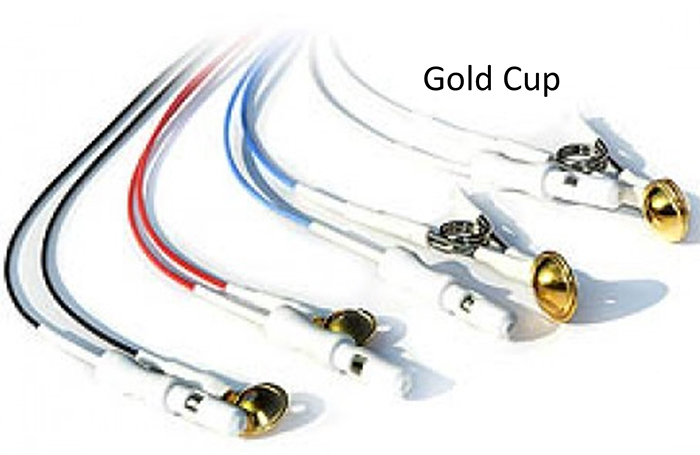
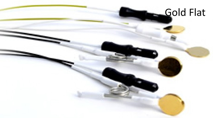
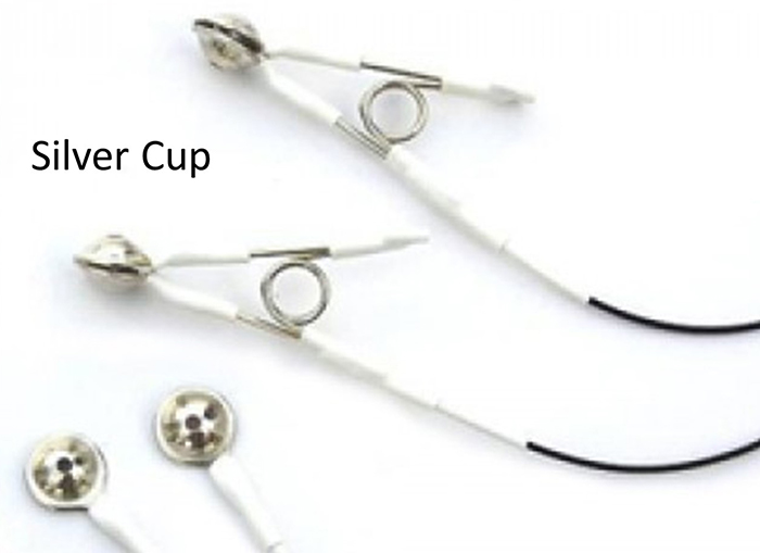
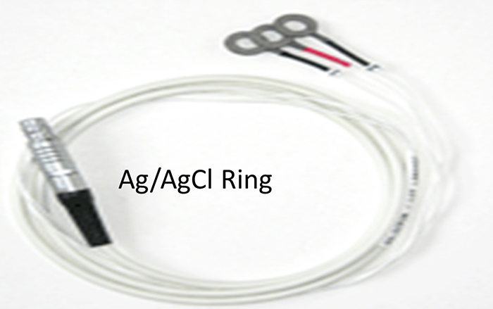
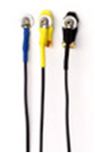
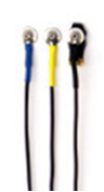
Electrodes detect biological signals. They are also transducers since they convert energy from one form to another. Four types of EEG electrodes are shown below: gold cup, gold flat, silver cup, and silver/silver-chloride ring.





 





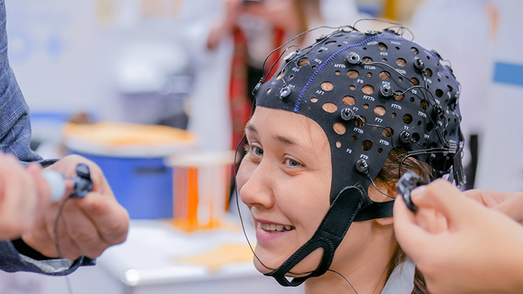
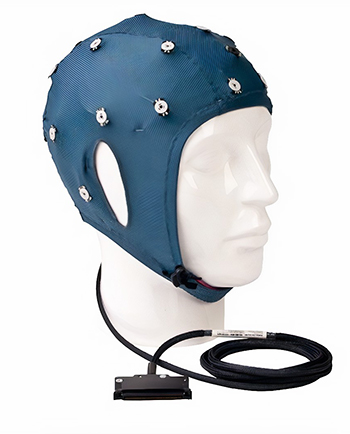
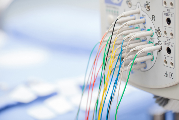
Cap systems like the NeXus EEG cap share a connector containing a pin or other type of connector for each electrode. These connectors plug all electrodes into the amplifier at the same time.




Consider how EEG electrodes work. In response to chemical and electrical synaptic messages, the dendrites of cortical pyramidal neurons develop excitatory postsynaptic potential (EPSPs) and inhibitory postsynaptic potentials (IPSPs) that travel about 10-12 centimeters as a current of ions through the cortex, blood vessels, glial cells, interstitial fluid, meninges, and skull to electrodes located on the scalp. This process is called volume conduction.


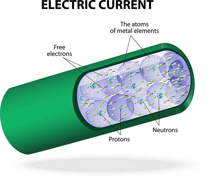
Electrodes transform this current of ions into a current of electrons that flows through the cable into an electroencephalograph’s input jack.





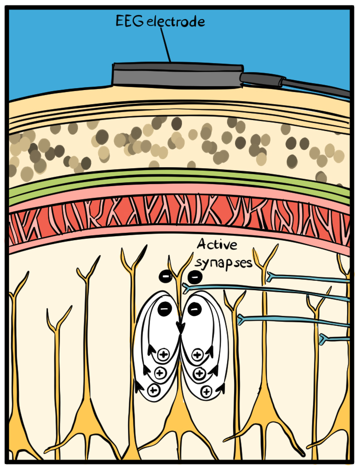
The EEG signal is attenuated during volume conduction. The volume-conducted signal that reaches EEG electrodes is measured in microvolts or millionths of a volt.

How do EEG electrodes work? When an EEG electrode is filled with a conductive gel or paste, the electrode metal donates ions to the electrolyte. In turn, the electrolyte contributes ions to the metal surface. Electrodes create a DC voltage between the electrode metal and the electroconductive gel or paste. Signal conduction succeeds as long as electrode and electrolyte ions are freely exchanged.

Recording Problems

Conduction breaks down during polarization when chemical reactions produce separate positive and negative charge regions where the electrode and gel make contact. DC flows across the connection between an electrode and the scalp. The current carries positive ions to the more negative region of this junction and negative ions to the more positive region. This build-up of ions polarizes the electrode to favor current flow in one direction and resists flow in the other.

When an electrode is polarized, ion exchange is reduced, and impedance increases, weakening the signal reaching the electroencephalograph. This problem can result from routine clinical use. Electrode manufacturers control this problem using silver/silver-chloride or gold electrodes that resist polarization.

Bias potentials are a second potential recording problem. They result from the exchange of metal ions donated by the electrodes and electrolytes in the absence of a biological current. Bias potentials can be prevented using electrodes with intact surfaces and identical materials (e.g., all gold or silver).

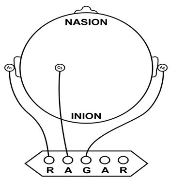
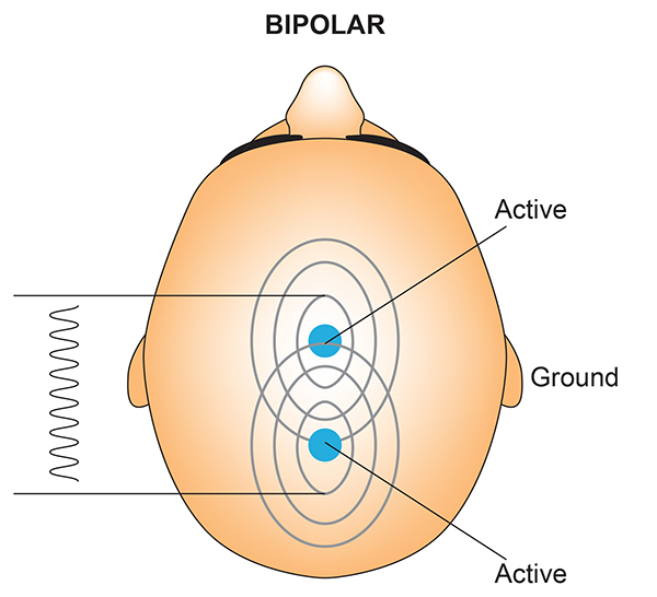
Recording the EEG with Three Leads

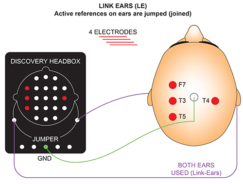
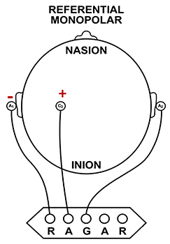
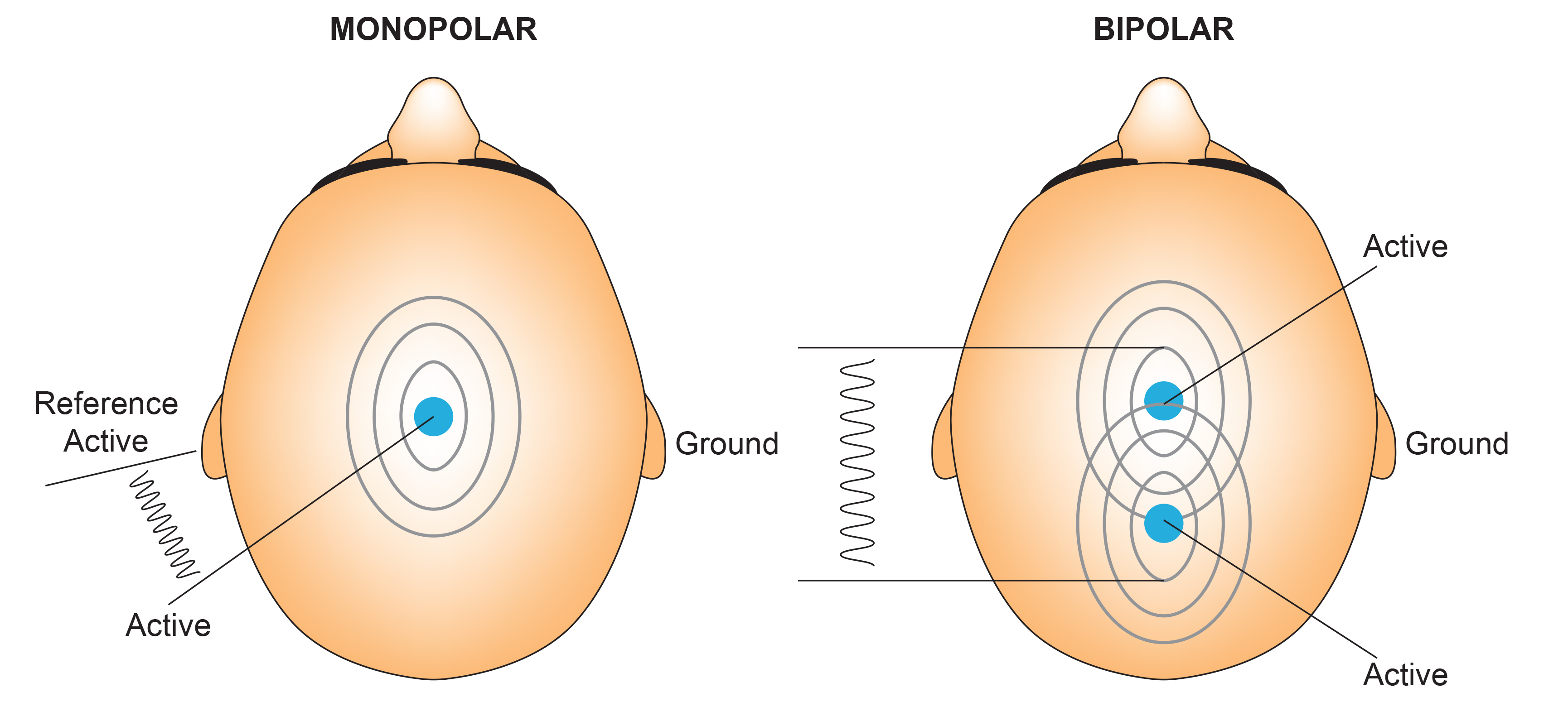
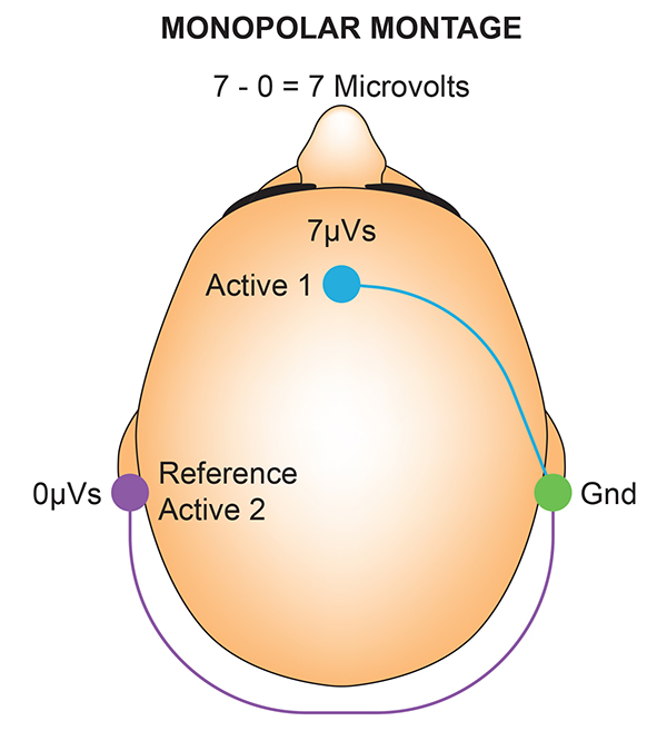
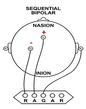
We record scalp electrical activity using three recording electrodes: active, reference, and ground. We place the active electrode over a scalp site, which is an EEG voltage source. We can locate the reference electrode over the scalp or neutral, but not electrically inactive, sites like an earlobe or the mastoid bone. Finally, we can place the ground electrode on an earlobe, mastoid bone, or scalp (Demos, 2019). The ground electrode is grounded to the amplifier.

Active and reference sensors are identical in construction and are each balanced inputs. They are interchangeable! However, some technologies require that you designate a sensor as a reference. For example, linked ears reference.

In the graphic below, the active (+) is red, the reference (-) is black, and the ground electrode (Gnd/Ref) is white.






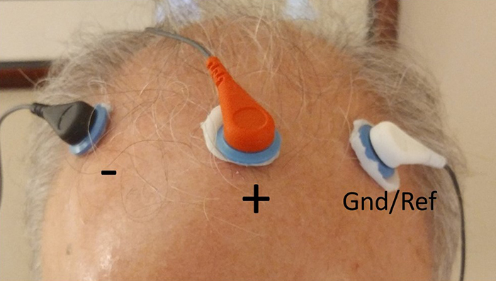
The voltages of the active and reference inputs are based on the ground.

EEG Apparatus

An electroencephalograph consists of the following stages: differential amplifier, gain amplifier, analog-to-digital converter, digital and FFT filters, and optical isolator.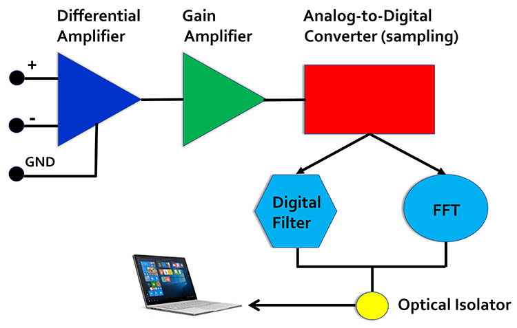

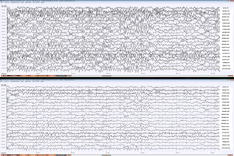
Signal Amplification

The biological signals monitored in biofeedback are very weak. The EEG signal, for example, is measured in microvolts (millionths of a volt). These signals must first be amplified over several stages to isolate the signal we are interested in and then drive displays. Stereo amplifiers perform the same tasks when they boost audio signals above the noise floor to levels that can power loudspeakers.

Amplifiers share the properties of input sensitivity and gain. Input sensitivity is the maximum voltage level an amplifier can accept without producing clipping and distortion. The graphic below shows the same EEG signal with different sensitivity. The top tracing shows greater sensitivity than the bottom tracing, as evidenced by its substantially greater voltage swings.





Gain is an amplifier's ability to increase the magnitude of an input signal to create a higher output voltage. Gain is the ratio of output/input, which is different for AC and DC systems. An amplifier that produces a 1-mV output from a 1-μV input has a gain of 1,000.

Differential Amplifiers

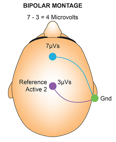
The EEG signal is first boosted by a differential amplifier and then by a gain amplifier. A differential amplifier, also called a balanced amplifier, amplifies the difference between the two inputs: the active (input 1) and reference (input 2). In the diagram below, the triangle represents the amplifier, and the black circles represent the input voltages. Graphic © Hand Robot/Shutterstock.com.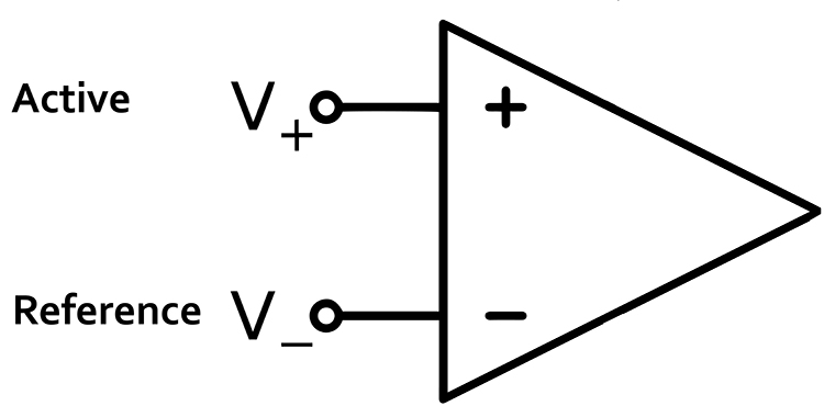




A differential amplifier combines two (or more) identical single-ended amplifiers with balanced inputs. The inputs are referenced to a common ground to compare the resulting signals. The amplifiers are 180o out of phase, so signals that differ in frequency, amplitude, and phase are amplified. Only signal components that differ between two inputs are retained and amplified as output. Signals that are out of phase or possess different amplitudes are "seen" by the common-mode rejection process as different and are retained.

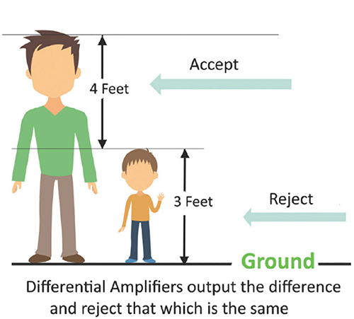
The graphic below was redrawn from John Demos' BCIA-recommended Getting Started with EEG Neurofeedback (2nd ed.). A differential amplifier rejects the common voltage (e.g., 3 feet) and outputs the voltage difference (e.g., 4 feet). A single-ended amplifier outputs the entire voltage (e.g., 7 feet, EEG artifact, and signal value).





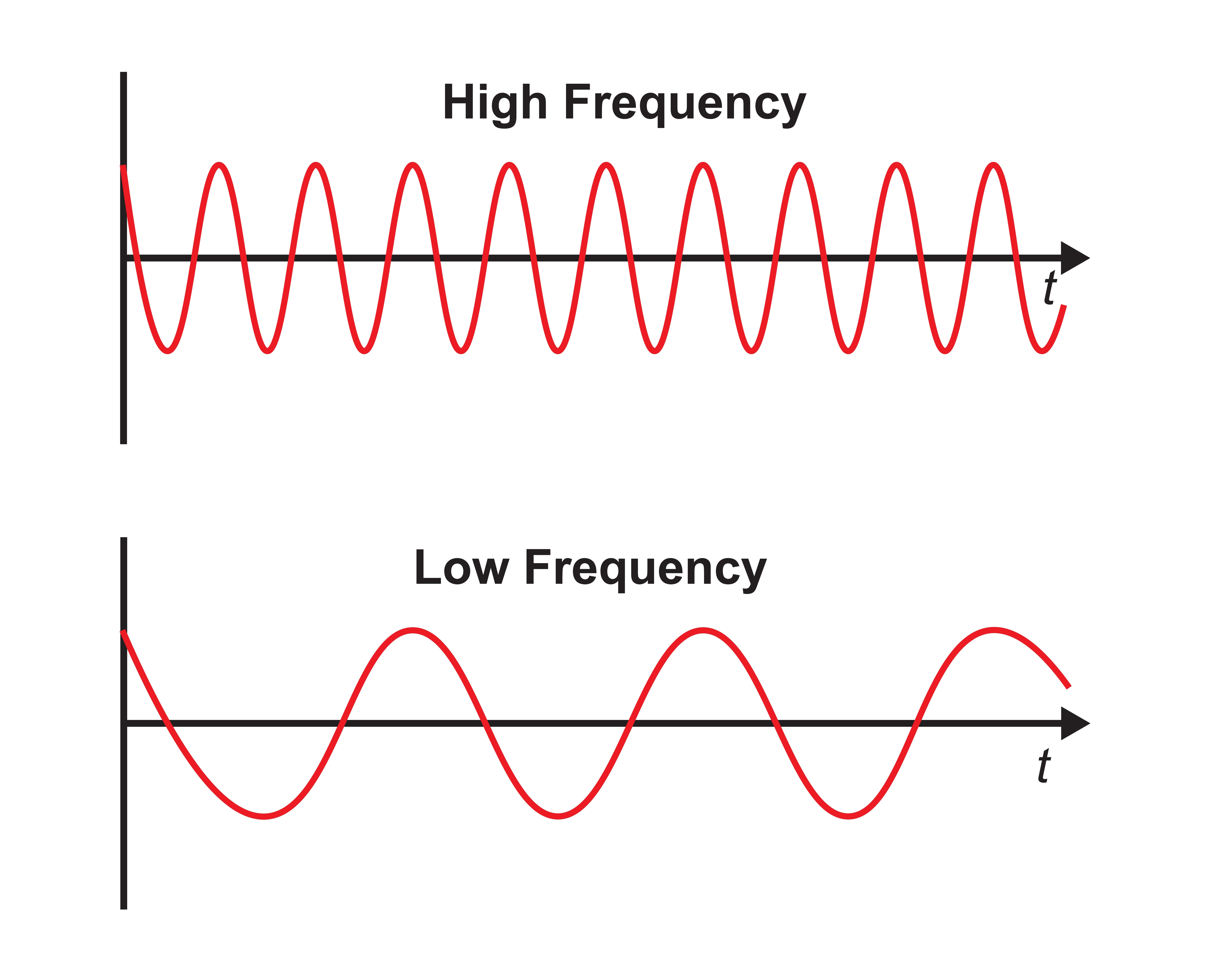
Frequency is the number of cycles per second (Hz). Frequency graphic © Bany's beautiful art/Shutterstock.com.



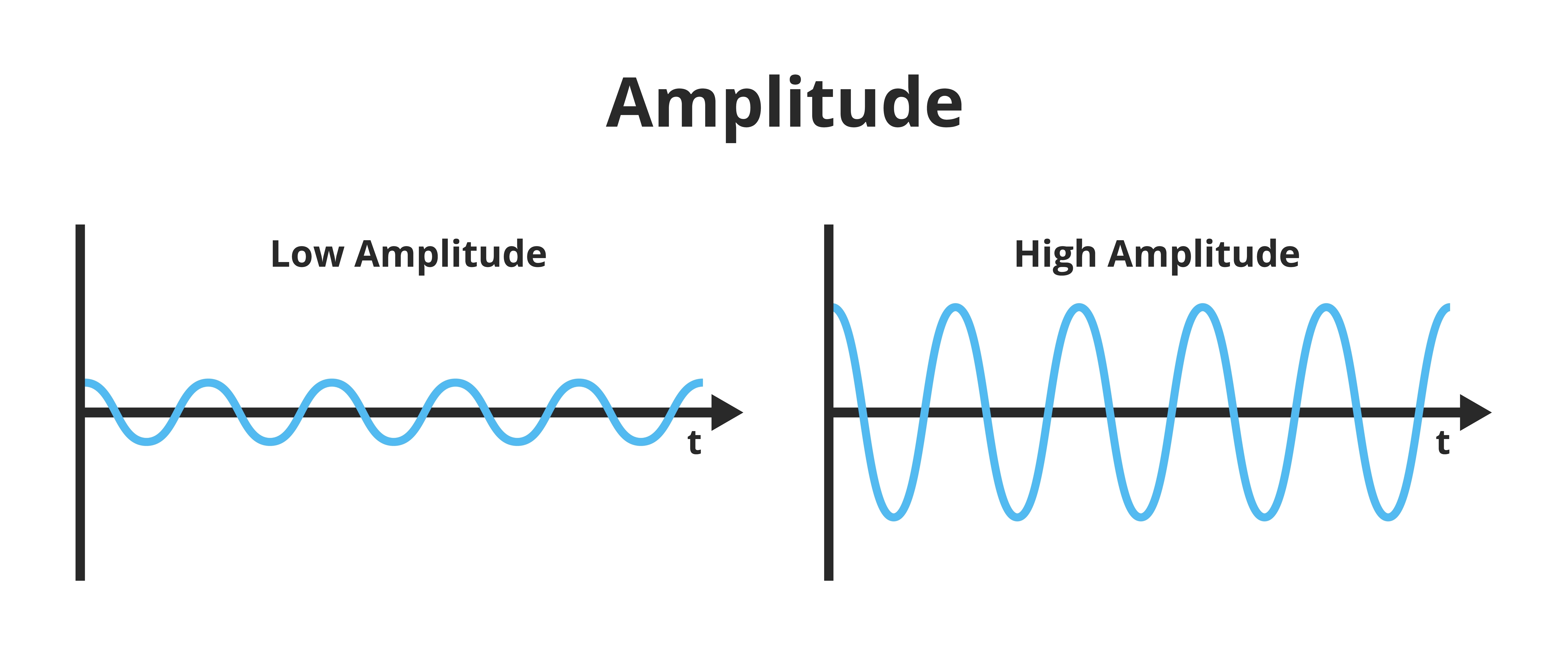
Amplitude is the signal voltage or power measured in microvolts or picowatts. Amplitude graphic © petrroudny43/Shutterstock.com.





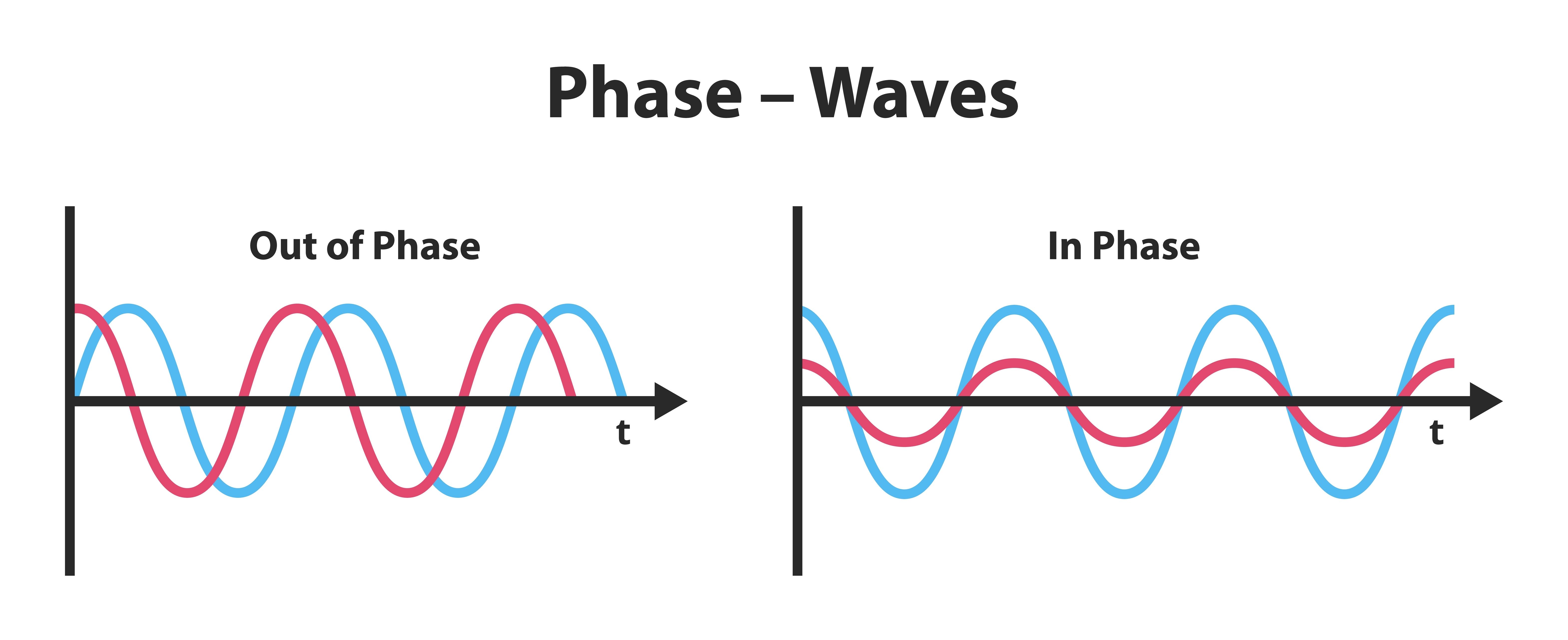
Phase is the similarity in timing of the waves at two locations. Note in the plot on the right. The two signals are 180^o out of phase so that the top signal peaks when the bottom signal reaches its trough. Phase graphic © petrroudny43/Shutterstock.com.




The recording below shows 4 tracings. The first one shows the Fp1 electrode referenced to linked ears and has an event circled in red. The second tracing shows the O2 electrode also referenced to linked ears and has a distinct EEG event circled in red. When the two electrodes, Fp1 and O2, are referenced (compared) to each other (the third tracing), the differences are retained, showing an example of common mode rejection (CMR). The fourth tracing shows the linked ears compared to each other, resulting in complete rejection of the identical signals. Typically, CMR occurs within the amplifier, although the resulting signals may be displayed in differing comparisons (montages) within the software, resulting in a similar function.




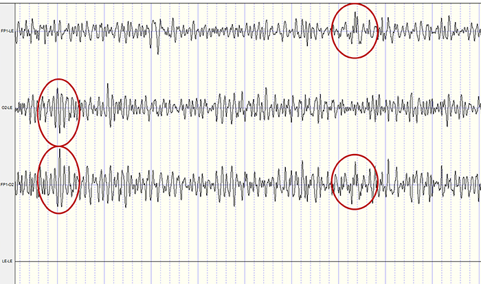
How does this reduce artifact? When there is no EEG activity, identical noise signals reach each amplifier. The differential amplifier subtracts these signals, canceling out the artifact. The output of a perfect differential amplifier would be 0.

The Challenges of Recording Infra-Slow EEG Activity

An AC amplifier has severe limitations when recording infra-slow (0-1 Hz) EEG activity. AC amplifiers exacerbate artifact effects. Client movement, eye movement, sweat, and transient field artifacts produce significant voltage changes. Long time constants over 80 s are recommended to integrate artifact-induced voltages over 2-4-min periods. However, persistent artifacts like eye movement will consistently degrade the signal-to-noise ratio of client feedback.

Infra-slow recording requires DC-coupled amplifiers with a large dynamic range produced by 24-bit A/D converters to prevent saturation by slow drifts in baseline voltage. Standard EEG electrodes made of gold, steel, or tin are unacceptable because they suffer capacitance or energy storage, blocking lower frequencies. Silver/silver-chloride electrodes are ideal because they are reversible and do not polarize.

The clinician must distinguish slow artifacts from infra-slow signals. Eccrine sweat glands produce standing millivolt-range potentials. While these can be eliminated by partial skin puncturing, this practice risks infection transmission. Clinicians can identify eye blink and eye movement artifacts by their characteristic location. Body tilt, cough and strain, hyperventilation, and tongue movements produce high amplitude diffuse very slow potentials (Miller et al., 2007).

Common-Mode Rejection

A differential amplifier’s separation of signal from artifacts is measured by the common-mode rejection ratio (CMRR). Since these amplifiers cancel out noise imperfectly, signal and noise will be boosted. The CMRR specification compares the degree to which a differential amplifier boosts signal (differential gain) and artifact (common-mode gain). CMRR = differential gain/common-mode gain.

CMRR should be measured at 50/60Hz where the strongest artifacts, like power line (50/60Hz) noise, are found. The smallest acceptable ratio is 100 dB (100,000:1), which means that the signal is boosted 100,000 times more than competing noise. State-of-the-art equipment exceeds a 180-dB ratio. Lower ratios could result in unacceptable contamination of biological signals.

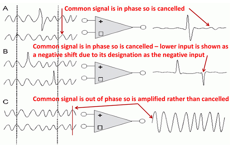
The graphic shows common-mode rejection when the common signal is in and out of phase.





You can take nine steps to maximize common-mode rejection:

(1) ensure that skin-electrode impedances are balanced within 1-3 Kohm. If both actives receive identical noise signals, the imbalance will make the signals look different and prevent complete subtraction of noise.

(2) active electrodes should be equidistant from the artifact source.

(3) active, reference, and ground sensors should be the same distance from each other.

(4) when using two or more channels, the ground and each active should be the same distance apart.

(5) ensure that there is a good ground connection. A deficient ground connection can make different voltages appear identical, defeating common-mode rejection.

(6) identify artifact sources. You can use a portable electroencephalograph or electromyograph like a Geiger counter. Move the unit around the room with EEG sensors connected but held in your hand. Artifact sources should produce the largest display values.

(7) remove the artifact sources you find. For example, fluorescent lights can be replaced with fixtures that produce less 50/60Hz noise.

(8) remove unused sensor cables from the encoder so they do not function as antennas for 50/60Hz artifacts.

(9) position the electroencephalograph and electrode cable to reduce artifact reception. Use the location and angle that yield the lowest readings when not attached to a patient (Thompson & Thompson, 2015).

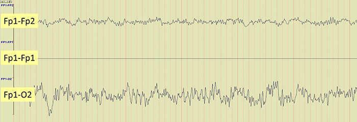
The Effect of Electrode Location on Common Mode Rejection

Brain activity is more similar when electrodes are close together and less similar when they are farther apart. A differential amplifier may reject actual EEG voltages detected by adjacent electrodes. The sensors were placed at the same anatomical location (Fp1-Fp1) for maximum cancellation, as shown by the flat line in the recording below.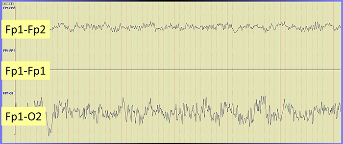

Differential Input Impedance

An amplifier’s differential input impedance further reduces the effect of unequal impedances. As EEG signals enter the amplifier, they are dropped across a network of resistors, presenting a differential input impedance in the Gohm (billion ohms) range. State-of-the-art instruments now exceed 10 Gohms. The differential input impedance must be at least 100 times skin-electrode impedance so that 99% or more of the signal can reach the electroencephalograph.

Why is this important? Stronger signals help an amplifier differentiate EEG activity from noise, producing more accurate feedback.

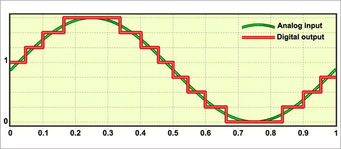
Sampling the EEG Signal

An analog-to-digital (A/D) converter samples the EEG signal at a fixed sampling interval. The sampling rate is the number of measurements taken within a given period. The sampling rate must be high enough to represent the measured signal accurately.

According to the Nyquist-Shannon sampling theorem, an A/D converter's sampling rate should be at least twice the highest frequency component you intend to sample.

The American Clinical Neurophysiology Society (ACNS) guidelines recommend a minimum sampling rate of at least three times the high-frequency filter setting for digitization. This means at least 100 samples per second (sps) for a 35-Hz high-pass filter and at least 200 sps for a 70-Hz high-pass filter (Halford et al., 2016).

A sampling rate of 128 sps is acceptable for visually inspecting the EEG. A rate of 256 sps is typical, and rates from 500-1000 sps are preferred. The graphic below shows the same EEG signal sampled at 32 and 256 sps. The vertical scale (signal amplitude) is identical for both rates.

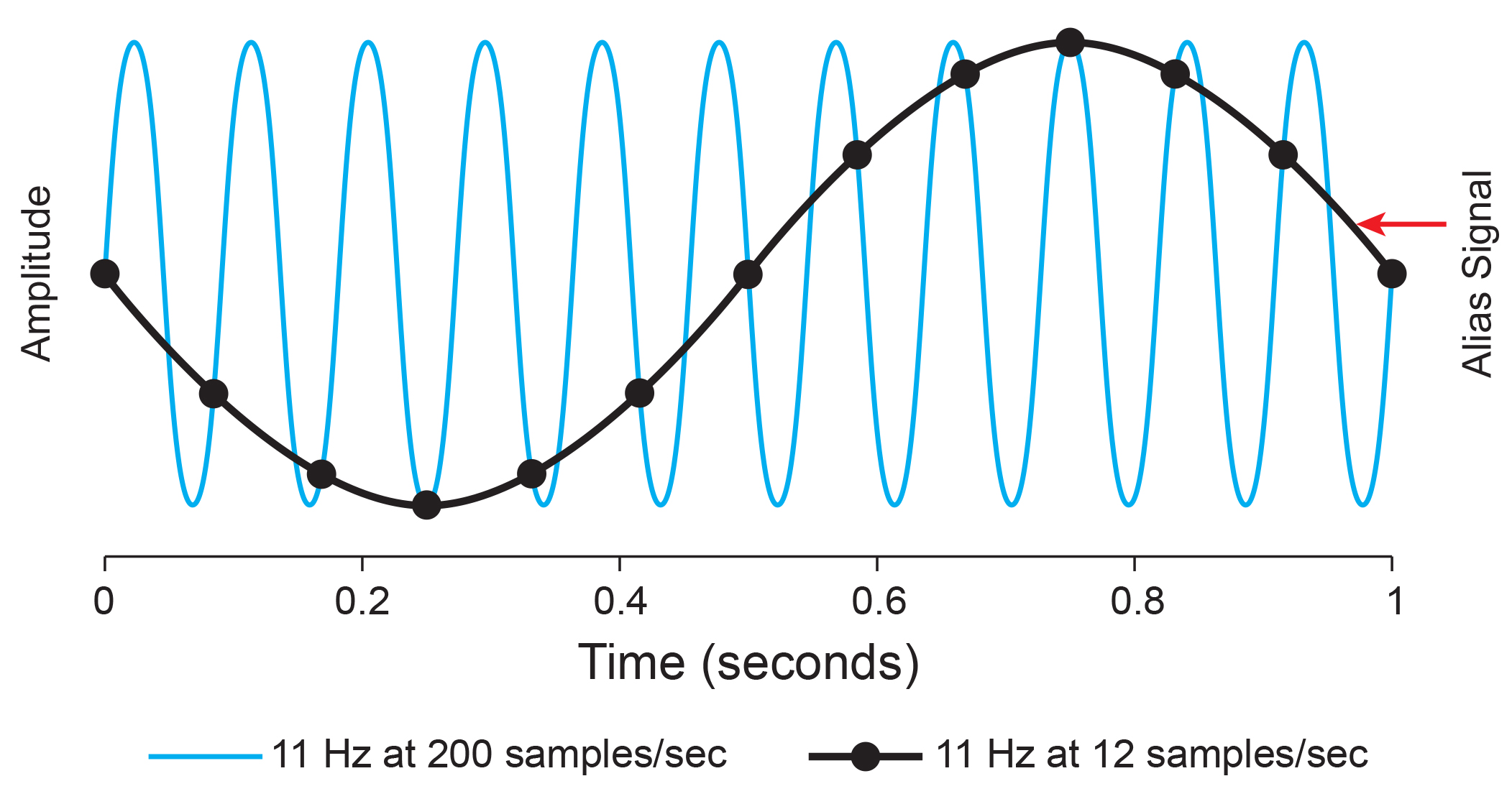
Sampling at too slow rates results in aliasing, where an analog signal seems to have a lower frequency than it does. "Phantom" slow activity results from too few samples per second. An 11-Hz signal is sampled at 12 and 200 sps. The 12-sps rate produces an aliasing signal shown in black. Graphic redrawn by minaanandag on Fiverr.com.

Resolution Depends on Bit Depth

An A/D converter's resolution is limited by the smallest signal amplitude it can sample. A bit number is the number of voltage levels an A/D converter can discern. ACNS (Halford et al., 2016) recommends a 16-bit resolution, which can discriminate among 65,536 voltage levels and achieve 0.05-μV resolution. Lower A/D converter resolutions overemphasize small voltage increases.

Signal Properties

EEG signals may be described by their frequency and amplitude. A/D conversion utilizes digital filters to break the EEG into its component frequencies. Prism graphic © kmls/Shutterstock.com.




The movie below is a 19-channel BioTrace+ /NeXus-32 display of EEG activity from 1-64 Hz activity broken into component delta, theta, alpha, and beta frequency bands by digital filters © John S. Anderson.




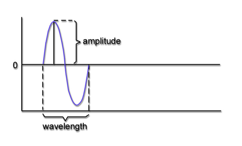
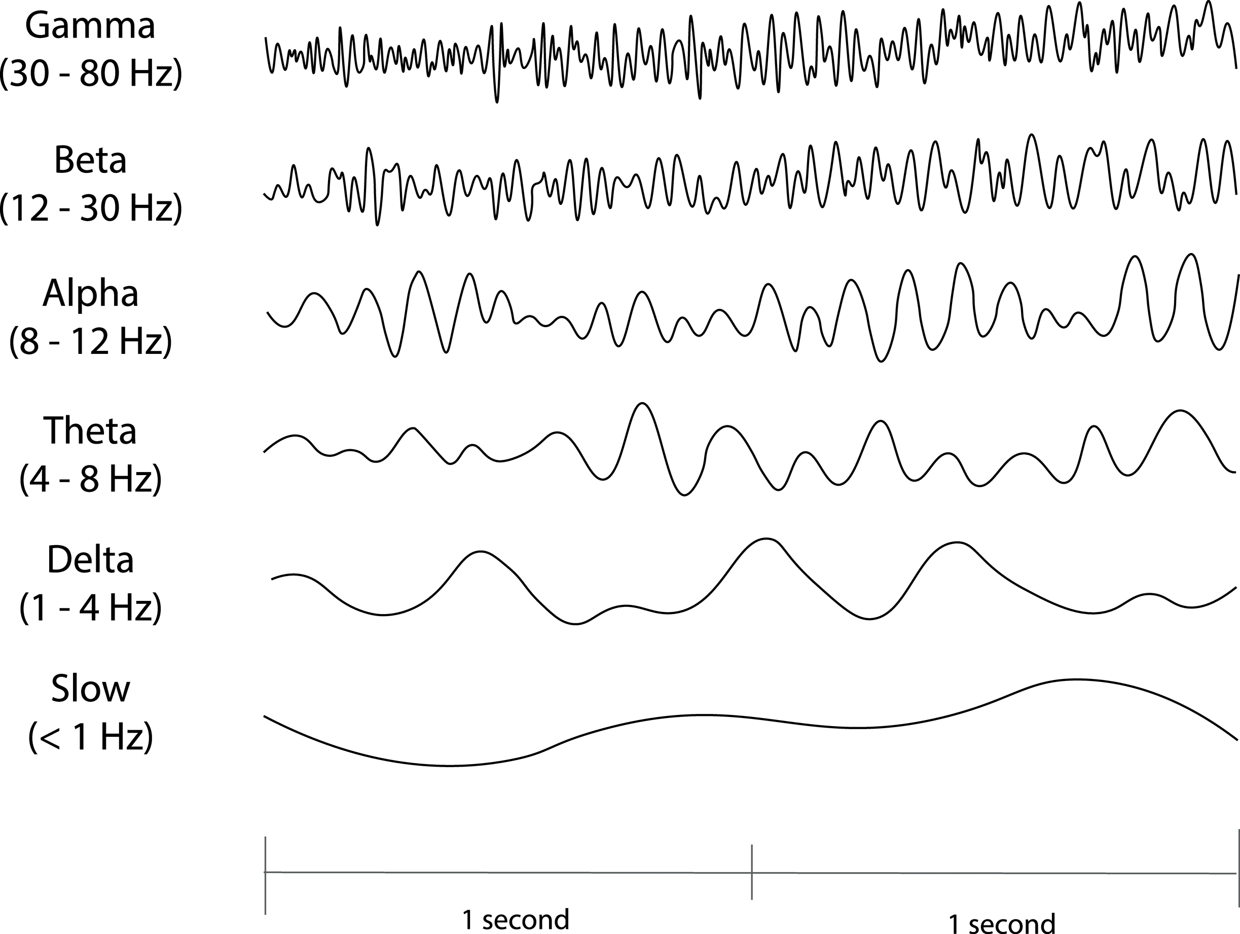
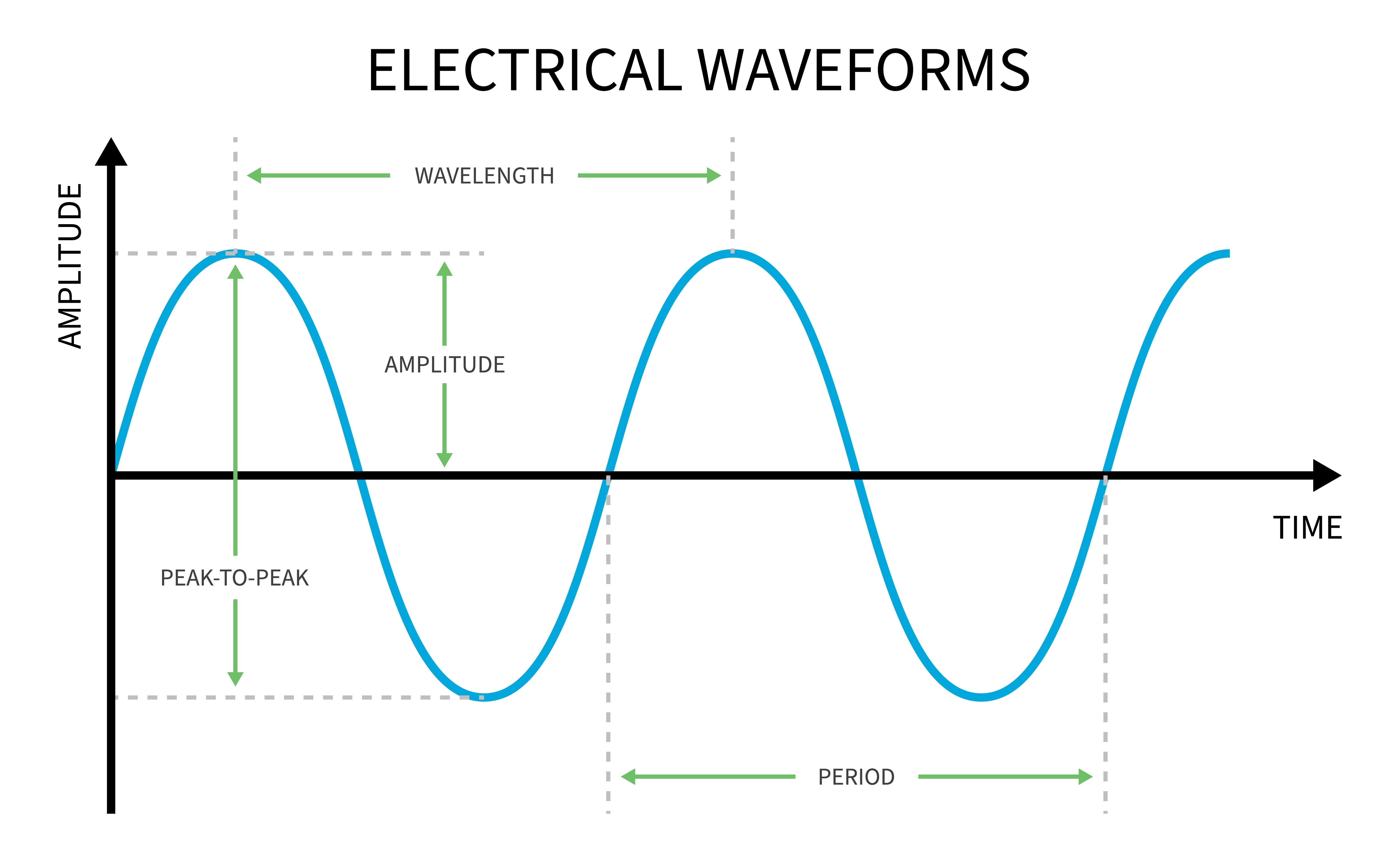
Recall that frequency is the number of cycles completed each second (Hz). The longer the wavelength, the slower the frequency. The delta, theta, alpha, and beta bands can be defined by wave frequency, wave shape or morphology, and context. EEG graphic © Jeniffer Fontan/Shutterstock.com.





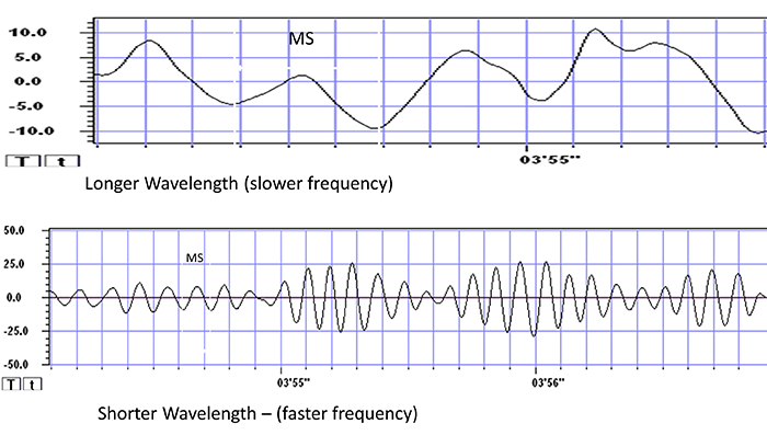
The next graphic illustrates the inverse relationship between wavelength and frequency. The time scale on the horizontal axis is in milliseconds. The amplitude scales are different for the upper (-10 to 10 μV) and lower (-50 to +50 μV) tracings.





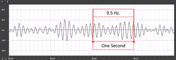
The graphic below shows a 9.5-Hz alpha wave. There are 9.5 peaks during a second.






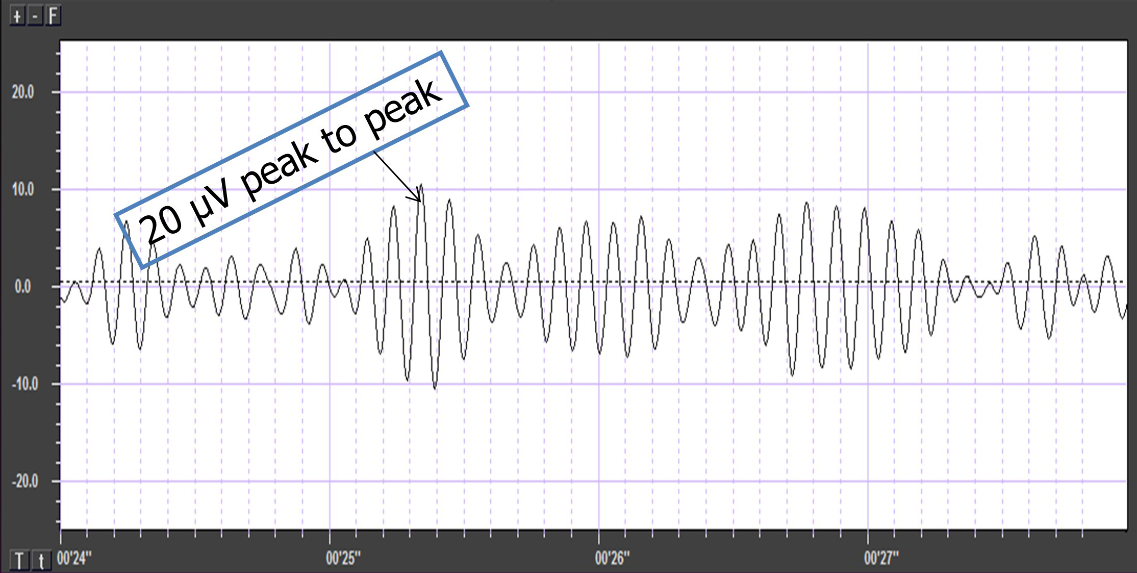
Also, recall that amplitude is signal voltage or power measured in microvolts or picowatts. The alpha wave below has a 20-μV amplitude.





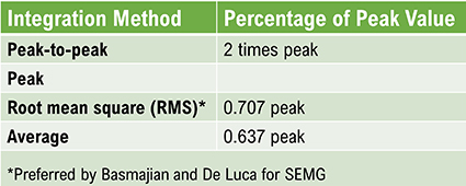
The EEG signal is sent to an integrator to measure signal amplitude in microvolts (μV) or picowatts. Integrators use four methods to calculate the voltage. The peak-to-peak method provides the largest estimate, equivalent to the energy contained between the positive and negative maximum values of the original AC waveform, which is 2 times the peak value. The peak voltage is 0.5 of the peak-to-peak value. The root mean square (RMS) voltage is 0.707 of the peak value and 20% higher than the average voltage. The average voltage is 0.637 of the peak value. Amplitude graphic © Pepermpron/Shutterstock.com.




Conversion among these methods is straightforward. If the peak-to-peak voltage is 20 μV, peak voltage is 10 μV, root mean square voltage is 7.07 μV, and average voltage is 6.37 μV.

Glossary

100 db: dB stands for decibel, a unit used to measure the intensity or level of sound, electrical signal, or other physical quantities. A decibel is a logarithmic unit that expresses the ratio of two values of a physical quantity. 100 dB represents a voltage level that is 100 times greater than the reference level,

active electrode: the electrode that is placed over a site that is a known EEG generator like Cz.

amplitude: signal strength measured in microvolts or picowatts.

analog-to-digital converter (ADC): an electronic device that converts continuous signals to discrete digital values.

bias potential: spurious voltage produced by the exchange of metal ions donated by the electrodes and electrolytes in the absence of a biological current.

bit number: the number of voltage levels that an A/D converter can discern. A resolution of 16 bits means that the converter can discriminate among 65,536 voltage levels.

common-mode rejection ratio (CMRR): the degree by which a differential amplifier boosts signal (differential gain) and artifact (common-mode gain).

differential amplifier (balanced amplifier): a device that boosts the difference between two inputs: the active (input 1) and reference (input 2).

differential input impedance: the opposition to an AC signal entering a differential amplifier as it is dropped across a resistor network.

digital filter: device that mathematically removes unwanted or extracts valuable aspects of a sampled, discrete-time signal.

electrode: a specialized conductor that converts biological signals like the EEG into currents of electrons.

frequency (Hz): the number of complete cycles that an AC signal completes in a second, usually expressed in hertz.

gain: an amplifier's ability to increase the magnitude of an input signal to create a higher output voltage; the ratio of output/input voltages.

ground electrode: a sensor placed on an earlobe, mastoid bone, or the scalp that is grounded to the amplifier.

input sensitivity: the maximum voltage level an amplifier can accept without producing clipping and distortion.

microvolt (μV): the unit of amplitude (signal strength) that is one-millionth of a volt.

Nyquist-Shannon sampling theorem: the perfect reconstruction of the analog signal requires sampling at two times its highest frequency. A signal whose highest frequency is 1000 Hz should be sampled

peak voltage: 0.5 of the peak-to-peak voltage.

peak-to-peak voltage: the voltage contained between the positive and negative maximum values of the original AC waveform.

phase: the degree to which the peaks and valleys of two waveforms coincide.

phase distortion: the displacement of the EEG waveform in time.

picowatt: billionths of a watt.

polarization: chemical reactions produce separate regions of positive and negative charge where an electrode and electrolyte make contact, reducing ion exchange.

power (W): the rate at which energy is transferred, which is proportional to the product of current and voltage. Power is measured in watts.

quantitative EEG (qEEG): digitized statistical brain mapping using at least a 19-channel montage to measure EEG amplitude within specific frequency bins.

reference electrode: the electrode placed over a less-electrically active site like the mastoid bone behind the ear.

resolution: degree of detail in a biofeedback display (0.1 μV) or the number of voltage levels an A/D converter can discriminate (16 bits or discrimination among 65,536 voltage levels).

sampling rate: the number of samples of a signal that are taken per second to represent the continuous signal digitally. It is measured in hertz (Hz) and is often denoted as samples per second (sps) or kilohertz (kHz).

volume conduction: the movement of biological signals through interstitial fluid.

volt (V): unit of electrical potential difference (electromotive force) that moves electrons in a circuit.

voltage (E): the amount of electrical potential difference (electromotive force).

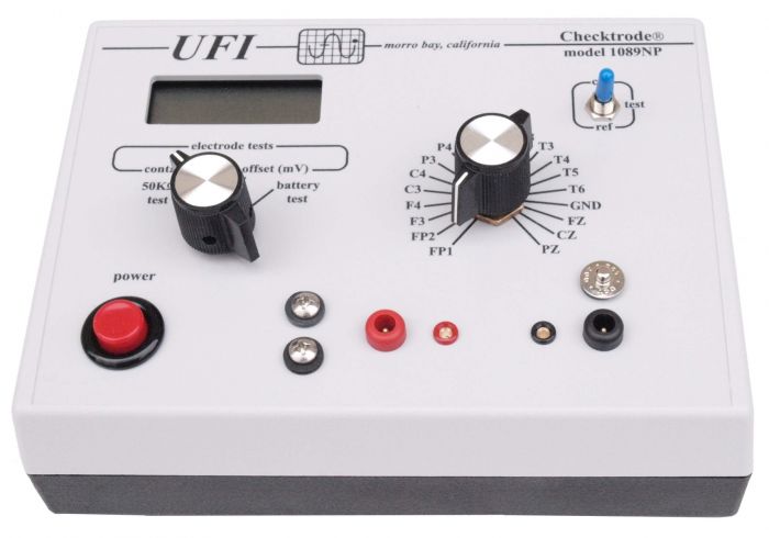
voltohmmeter: a device that uses a DC signal to measure resistance in an electric circuit, such as between active and reference electrodes.

watt (W): a unit of power used to express signal strength in the qEEG.

TEST YOURSELF ON CLASSMARKER

Click on the ClassMarker logo below to take a 10-question exam over this entire unit.

REVIEW FLASHCARDS ON QUIZLET

Click on the Quizlet logo to review our chapter flashcards.

Visit the BioSource Software Website

BioSource Software offers Physiological Psychology, which satisfies BCIA's Physiological Psychology requirement, and Neurofeedback100, which provides extensive multiple-choice testing over the Biofeedback Blueprint.

Assignment

Now that you have completed this module, explain why bit-depth and sampling rate matter.

References

Andreassi, J. L. (2000). Psychophysiology: Human behavior and physiological response. Lawrence Erlbaum and Associates, Inc.

Basmajian, J. V. (Ed.). (1989). Biofeedback: Principles and practice for clinicians. Williams & Wilkins.

Cacioppo, J. T., & Tassinary, L. G. (Eds.). (1990). Principles of psychophysiology. Cambridge University Press.

Collura, T. F. (2014). Technical foundations of neurofeedback. Taylor & Francis.

Demos, J. N. (2005). Getting started with neurofeedback. W. W. Norton & Company.

Fisch, B. J. (1999). Fisch and Spehlmann's EEG primer (3rd ed.). Elsevier.

Floyd, T. L. (1987). Electronics fundamentals: Circuits, devices, and applications. Merrill Publishing Company.

Grant, A. (2015). Four elements earn permanent seats on the periodic table. Science News.

Halford, J. J., Sabau, D., Drislane, F. W., Tsuchida, T. N., & Sinha, S. R. (2016). American Clinical Society Guideline 4: Recording clinical EEG on digital media. Journal of Clinical Neurophysiology, 33(4), 317-319. https://doi.org/10.1080/21646821.2016.1245563

Hughes, J. R. (1994). EEG in clinical practice (2nd ed.). Butterworth-Heinemann.

Kubala, T. (2009). Electricity 1: Devices, circuits, and materials (9th ed.). Cengage Learning.

Libenson, M. H. (2010). Practical approach to electroencephalography. Saunders Elsevier.

Miller, J. W., Kim, W. S., Homes, M. D., & Vanhatalo, S. (2007). Ictal localization by source analysis of infraslow activity in DC-coupled scalp EEG recordings. NeuroImage, 35(2), 583-597. https://doi.org/10.1016/j.neuroimage.2006.12.018

Montgomery, D. (2004). Introduction to biofeedback. Module 3: Psychophysiological recording. Association for Applied Psychophysiology and Biofeedback.

Nilsson, J. W., & Riedel, S. A. (2008). Electric circuits (8th ed.). Pearson Prentice-Hall.

Peek, C. J. (2016). A primer of traditional biofeedback instrumentation. In M. S. Schwartz, & F. Andrasik (Eds.). (2016). Biofeedback: A practitioner's guide (4th ed.). The Guilford Press.

Stern, R. M., Ray, W. J., & Quigley, K. S. (2001). Psychophysiological recording (2nd ed.). Oxford University Press.

Thompson, M., & Thompson, L. (2015). The biofeedback book: An introduction to basic concepts in applied psychophysiology (2nd ed.). Association for Applied Psychophysiology and Biofeedback.

Wadman, W. J., & Lopes da Silva, F. H. (2011). In D. L. Schomer & F. H. Lopes da Silva (Eds.). Niedermeyer's electroencephalography: Basic principles, clinical applications, and related fields (6th ed.). Lippincott Williams & Wilkins.

C. Instrumentation (Acquisition and Review Parameters/Settings)

Quantitative Electroencephalography (qEEG) is a powerful tool in neuropsychology and neuroscience for analyzing the brain's electrical activity. Ensuring accurate and reliable data collection involves several critical parameters and settings.

Please click on the podcast icon below to hear a full-length lecture over Section C.

First, electrode placement and the number of electrodes are fundamental. Standardized placement using the International 10-20 or 10-10 system is essential for consistent and reproducible electrode locations across subjects and sessions (Klem et al., 1999). Typically, a high-density cap with 19, 32, 64, or more electrodes captures detailed spatial information (Nuwer, 1997).

Second, the sampling rate is another crucial parameter. The minimum sampling rate should be at least 256 Hz, but higher rates, such as 512 Hz or 1024 Hz, are preferred for capturing fast neural dynamics and avoiding aliasing (Miller et al., 2009).

Third, data acquisition settings also play a vital role. Filter settings should include a high-pass filter set around 0.5-1 Hz and a low-pass filter set around 70-100 Hz to remove artifacts and noise outside the frequency range of interest (Luck, 2014). A 50/60 Hz notch filter should also be applied to eliminate power line noise, depending on the regional electrical supply frequency.

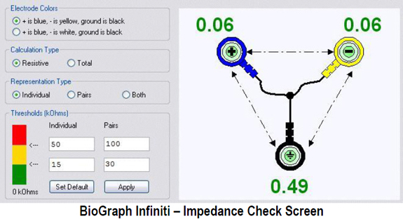
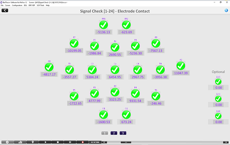
Fourth, maintaining low impedance levels is essential for signal quality. Electrode impedances should be kept below 5 kΩ to ensure good signal quality and reduce artifacts, with lower impedance values preferable (Ferree et al., 2001).

Fifth, artifact management is another critical aspect of qEEG. Implementing real-time artifact rejection algorithms can help exclude segments contaminated by eye movements, muscle activity, or electrical noise. Post-processing methods, such as Independent Component Analysis (ICA), are useful for artifact correction (Jung et al., 2000).

Sixth, the choice of reference electrode can significantly affect the results. Common references include linked earlobes, mastoids, or an average reference, and this choice should be consistent across subjects and sessions (Yao, 2001).

Seventh, the recording environment should be controlled to minimize environmental noise and ensure subject comfort. This includes performing recordings in a quiet, electrically shielded room with controlled temperature and lighting.

Finally, proper subject preparation is essential for accurate qEEG data. Subjects should avoid caffeine, heavy meals, and intense physical activity before the recording session. Ensuring they are well-rested and relaxed can help reduce movement artifacts.

These settings and parameters are critical for obtaining high-quality qEEG data, which can provide valuable insights into brain function and dysfunction.

The movie below shows parameters and settings when processing a 19-channel EEG recording in NeuroGuide © John S. Anderson.

EEG Filters Define the Signal

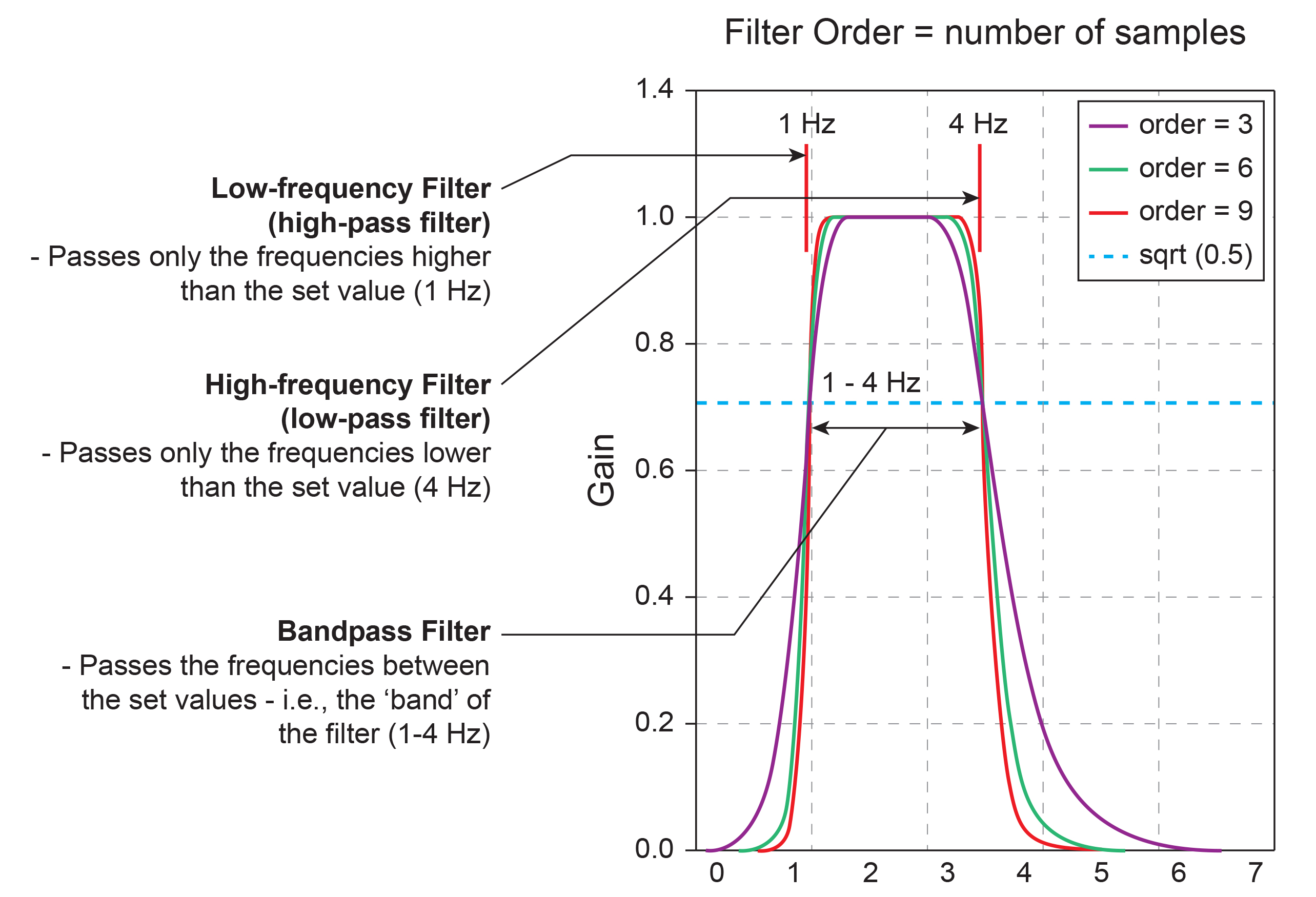
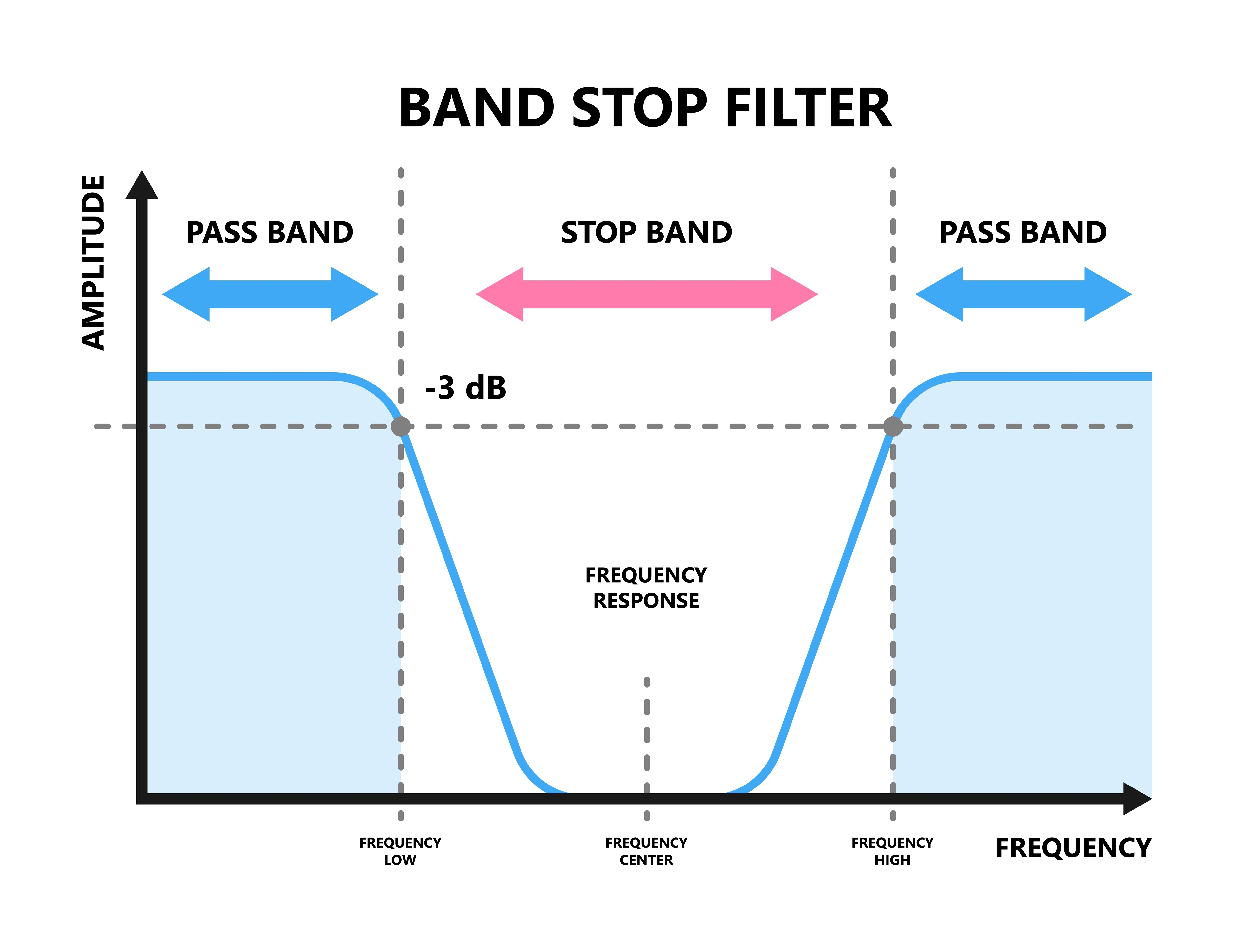
EEG filters select signals of interest and minimize artifacts. In this section, we will review high-pass, low-pass, bandpass, and notch filters. In the graphic below, the range of frequencies passed through a filter is called the passband, and the range that is sharply attenuated is called the stopband. Filter graphic redrawn by minaanandag at Fiverr.com.





A high-pass filter only passes frequencies higher than a set value (e.g., 1 Hz). A low-pass filter only passes frequencies lower than a specified value (e.g., 40 Hz). A bandpass filter passes frequencies between the set values, the "band" of the filter (e.g., 1-40 Hz). Graphic redrawn by minaanandag at Fiverr.com.




10-Hz Low-Pass Filter

The movie below shows the output of a 10-Hz low-pass filter with a vertical scale of 0-50 μV © John S. Anderson.




20-Hz Low-Pass Filter

The movie below shows the output of a 20-Hz low-pass filter with a vertical scale of 0-50 μV © John S. Anderson.





30-Hz Low-Pass Filter

The movie below shows the output of a 30-Hz low-pass filter with a vertical scale of 0-50 μV © John S. Anderson.





40-Hz Low-Pass Filter

The movie below shows the output of a 40-Hz low-pass filter with a vertical scale of 0-50 μV © John S. Anderson.





10-Hz High-Pass Filter

The movie below shows the output of a 10-Hz high-pass filter with a vertical scale of 0-50 μV © John S. Anderson.




20-Hz High-Pass Filter

The movie below shows the output of a 20-Hz high-pass filter with a vertical scale of 0-50 μV © John S. Anderson.





30-Hz High-Pass Filter

The movie below shows the output of a 30-Hz high-pass filter with a vertical scale of 0-50 μV © John S. Anderson.