Signal Acquisition

Clinicians monitor EEG activity using the classical International 10-20 System for standardized electrode placement or the modified "10-10" system known as the Modified Combinatorial Nomenclature System. They often record from several sites and measure the amplitude of EEG signals within frequency bands (like alpha and theta) to provide a complete picture of brain activity. Software-based montage reformatting allows clinicians to reanalyze session data by referencing an electrode to other sites or combinations of sites. This system also allows for the computation of multiple variables associated with communication and network functions within the central nervous system (CNS)

The Quantitative EEG (qEEG) measures EEG amplitudes within selected frequency bands. A full-cap 21-channel EEG recording (19 scalp sensors plus two "reference" sensors) and resulting qEEG analysis may be valuable in designing treatment protocols for complicated cases like Asperger's or traumatic brain injury. EEG topography displays the qEEG on a cortical surface map to show the spatial distribution of EEG activity.

Contamination of the EEG by physiological and exogeneous artifacts requires that clinicians take extensive precautions, examine the raw EEG record, and remove contaminated epochs through artifacting. Impedance tests and behavioral tests help ensure the fidelity of EEG recording.

Finally, clinicians interpret EEG recordings with an understanding of normal values and recognition of the effects of eye closure, age, diurnal influences, alertness and drowsiness, medication, and relaxation on these readings. Graphic © Medical-R/Shutterstock.com.

BCIA Blueprint Coverage

This unit addresses III. Instrumentation and Electronics - B. Signal Acquisition.



This unit covers International 10-20 and 10-10 Systems, Comparison of Neuroimaging Techniques, Using a Limited Number of Electrodes, Montage Options and Their Consequences, Recognizing and Correcting Signals of Noncerebral Origin, and Recognizing Normal EEG Patterns.

Please click on the podcast icon below to hear a lecture over the first half of this unit.

International 10-20 and 10-10 Systems

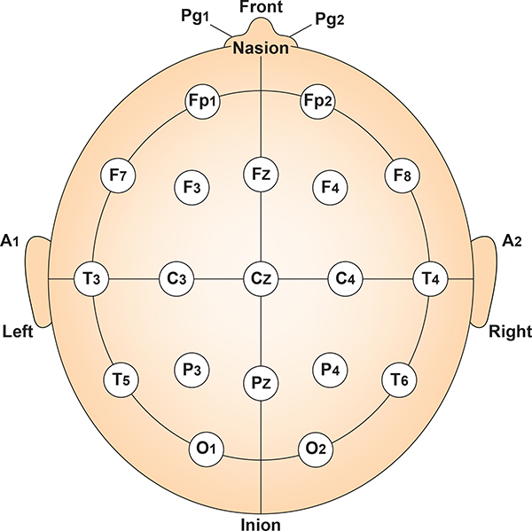
The International 10-20 system is a standardized procedure for electrode placement on 19 scalp and reference and ground sites. Electrodes measure electrical activity from a surrounding area the size of a quarter. The site recorded may be distant from the EEG generator due to neural pathways.




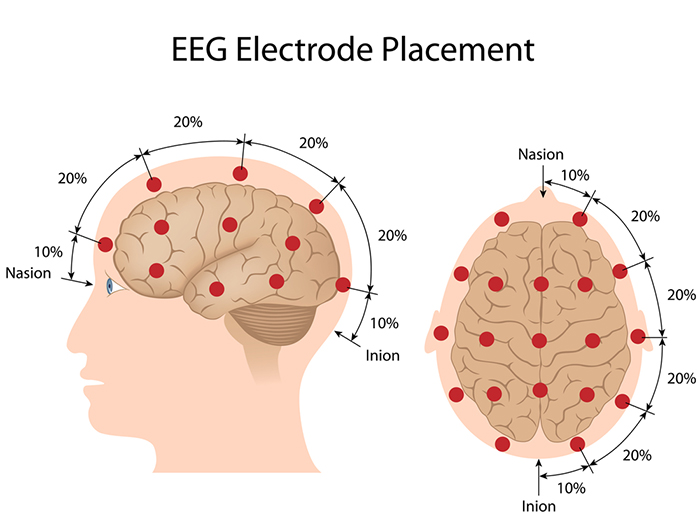
The International 10-20 system calculates the distance between the nasion to the inion and the left preauricular notch to the right preauricular notch. The 19 active electrode positions are found taking either 10% or 20% of these distances. Check out the YouTube video The International 10-20 System. Four essential landmarks are the nasion, inion, preauricular points, and vertex. Graphic © Alila Medical Media/Shutterstock.com.




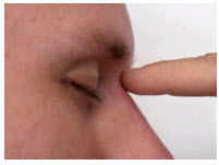
The nasion is the depression at the bridge of the nose.




The inion is the bony prominence on the back of the skull in the middle of the inion ridge.





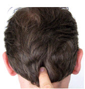
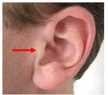
The left and right preauricular points are slight depressions located in front of the ears and above the earlobe. The flap at the opening of the ear is called the tragus.






The vertex (Cz) intersects imaginary lines drawn from the nasion to inion and between the two preauricular points. Cz is 50% between the nasion and inion and 50% between the two preauricular points. Minaanandag adapted the diagram below from Fisch (1999).






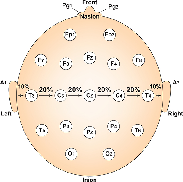
The 10-20 system received its name because electrode sites are separated by 10% or 20% of the distance between two corresponding anatomical landmarks. In the graphic below adapted from Fisch (1999) by minaanandag, each midline site is 10% or 20% of the distance from the nasion to the inion.






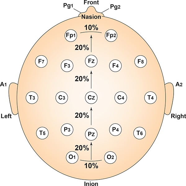
Each horizontal axis site is 10% or 20% of the distance from the two preauricular points. Graphic adapted from Fisch (1999) by minaanandag.




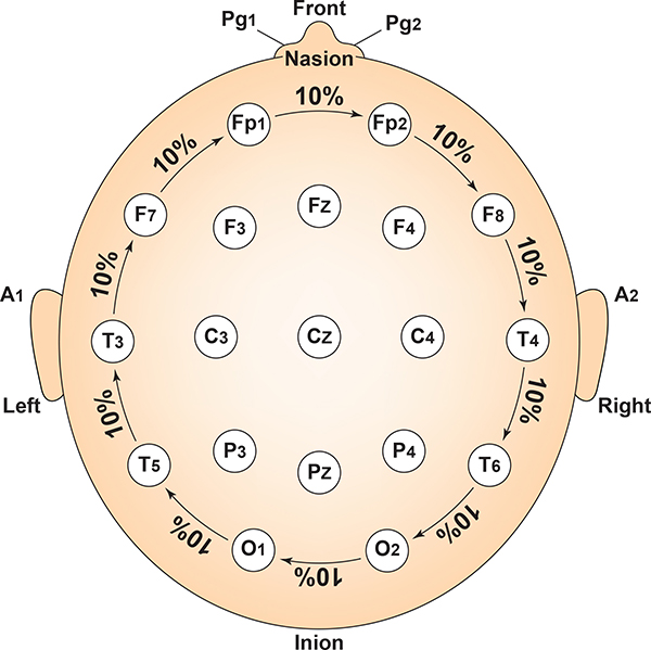
Each circumferential site is 10% of the total circumference, excluding Fpz or Oz. Graphic adapted from Fisch (1999) by minaanandag.






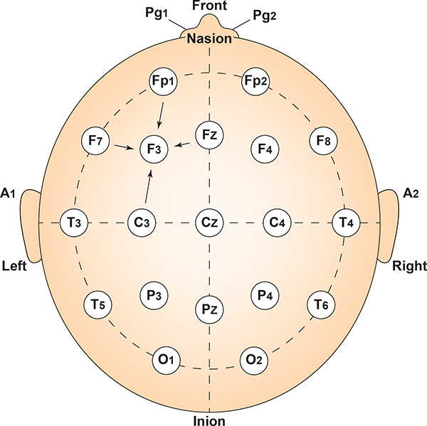
Intermediate sites are halfway between sets of adjacent sites. Graphic adapted from Fisch (1999) by minaanandag.







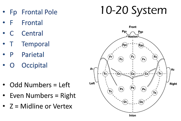
The 10-20 system assigns recording electrodes a letter and subscript. The letters represent the underlying region and include Fp (frontopolar or prefrontal), F (frontal), C (central), P (parietal), O (occipital), and A (auricular). A subscript of z represents a midline (central axis from nasion to inion) placement.

Numerical subscripts range from 1-8 and increase with distance from the midline. The 10-20 system assigns odd-numbered recording electrodes on the left and even-numbered electrodes on the right side of the head. Two reference electrodes are usually placed on the earlobe. John Balven adapted the diagram below from Fisch (1999).

Modified Combinatorial Nomenclature

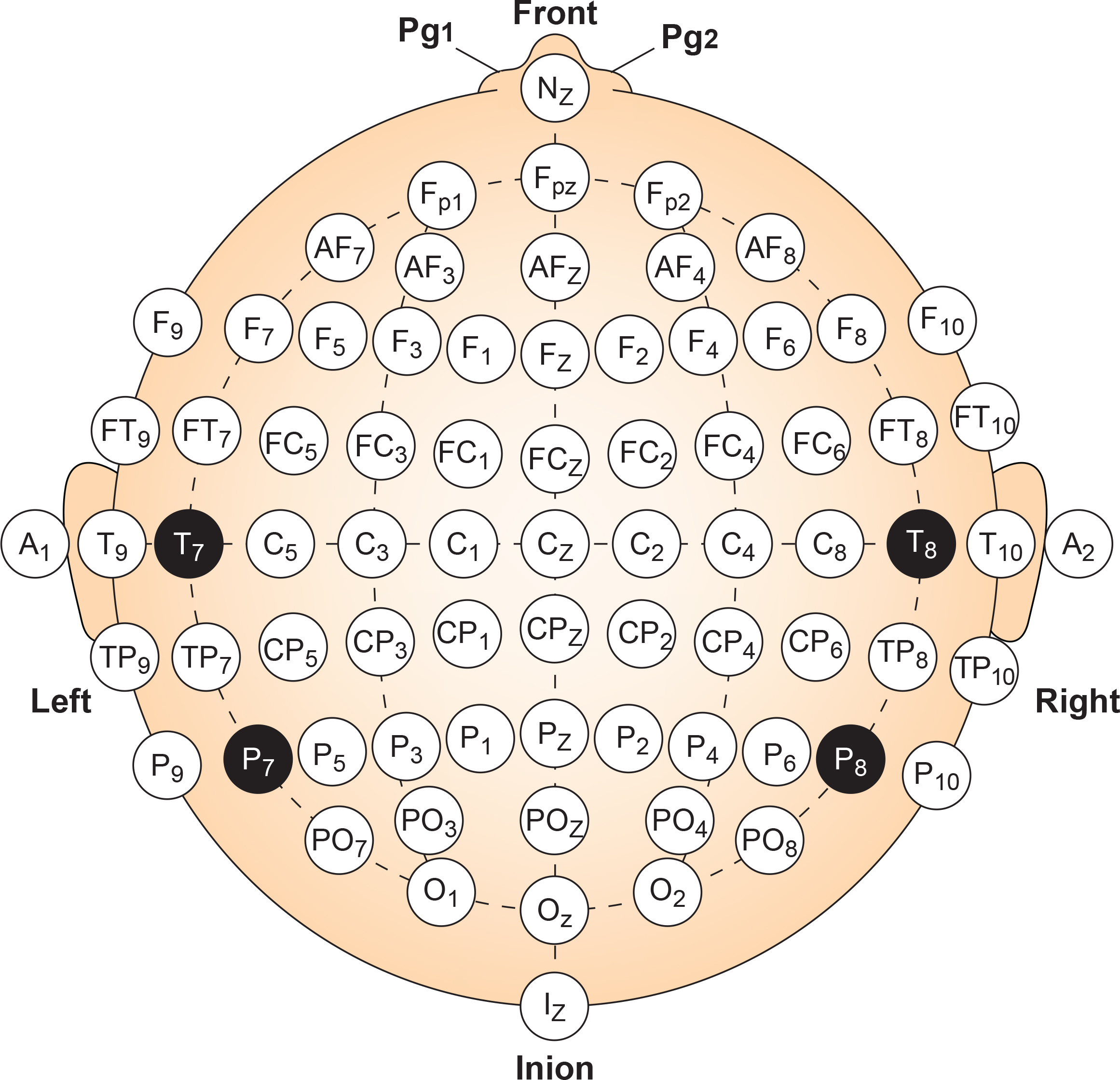
The American Clinical Neurophysiology Society published guidelines for expanding the 10-20 system to 75 electrode sites. This system, while more complex, also allows us to precisely define the placement sites for our electrodes.

The expansion of the 10-20 system allows clinicians to define the sites midway between two 10-20 sites commonly used in clinical practice, better localize epileptiform activity, increase EEG spatial resolution, and improve detection of localized evoked potentials. The modified combinatorial system replaces inconsistent designations (T3/T4 and T5/T6) with consistent ones (T7/T8 and P7/P8). Black circles depict these replacement sites with white lettering in the diagram below.

The modified combinatorial system, also called the 10-10 system, locates electrodes at every 10% along medial-lateral contours and adds new contours. Each electrode site intersects a medial-to-lateral coronal line (designated by letters) and a longitudinal sagittal line (designated by numerical subscripts).

As with the 10-20 system, letters represent the underlying region.



N (nasion), Fp (frontopolar or prefrontal), AF (anterior frontal), F (frontal), FT (frontotemporal), FC (frontocentral), A (auricular), T (temporal), C (central), TP (temporal-posterior temporal), CP (centroparietal), P (parietal), PO (posterior temporo-occipital or parieto-occipital), O (occipital), and I (inion). FT and FC lie along the second intermediate coronal line, TP and CP along the third, and PO along the fourth.

A subscript of z represents a midline (central axis from nasion to inion) placement. Numerical subscripts range from 1-10 and increase with distance from the midline. The modified combinatorial system assigns odd-numbered recording electrodes on the left and even-numbered electrodes on the right side of the head. David Kelsey adapted the diagram below from Fisch (1999).

Comparison of Neuroimaging Techniques

Neuroimaging methods can be thought of as either structural or functional. Structural methods include CT and MRI and present images of brain structures. Functional methods include EEG, MEG, fMRI, PET, and SPECT, each of which constructs images showing the location of differing levels of brain activity.

The different functional neuroimaging methods use different biologic signals as their index of function. EEG and MEG use brain electrical activity, fMRI uses blood oxygen level, PET uses positron-emitting radioisotopes bound to glucose, and SPECT uses gamma-emitting radioisotopes. Therefore, PET and SPECT are more invasive and pose more significant risks to patients and research participants (Breedlove & Watson, 2023).

Each functional neuroimaging method can be rated with respect to how quickly it can detect changes in function (temporal resolution) and over how small an area it detects changes in function (spatial resolution). Whereas EEG and MEG methods detect changes in function most quickly, they are less able to detect the precise area where functional changes occur compared to fMRI. Graphic redrawn by minaanandag at Fiverr.com.

STRUCTURAL TECHNIQUES

The main structural imaging techniques are computerized axial tomography and magnetic resonance imaging.

Computerized Axial Tomography

Computerized Axial Tomography (CAT or CT) provides medium-resolution images of brain structure by moving an x-ray source along an arc surrounding the head (Breedlove & Watson, 2023). Graphic © Tyler Olson/Shutterstock.com.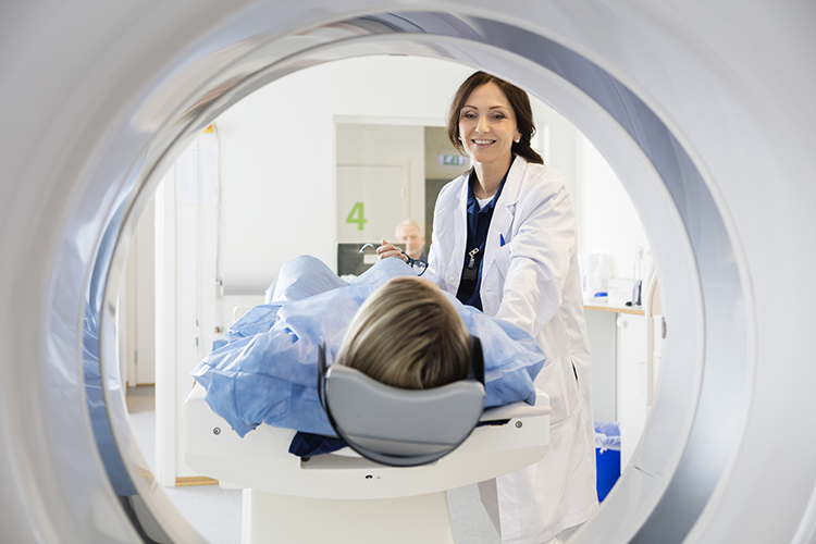




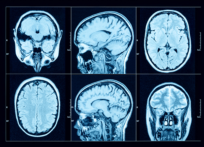
CT scans allow physicians to visualize structural abnormalities like stroke damage and tumors. Graphic © Triff/Shutterstock.com.

Magnetic Resonance Imaging (MRI)

Magnetic resonance imaging (MRI) constructs higher-resolution images than CT scans. Since MRI scans use powerful magnetic fields and radio wave pulses to construct images of living brains, they are safer than CT scans because there is no radiation exposure. MRI scans allow a detailed examination of brain topography, including the location and volume of specific brain regions. Graphic © Peastock/Shutterstock.com.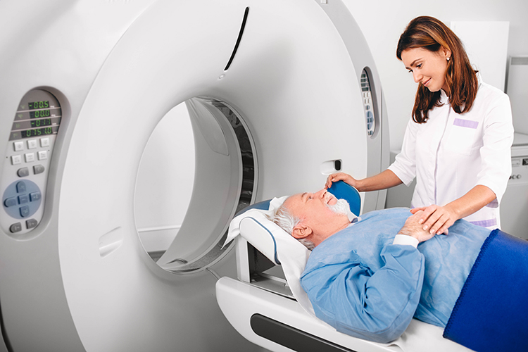





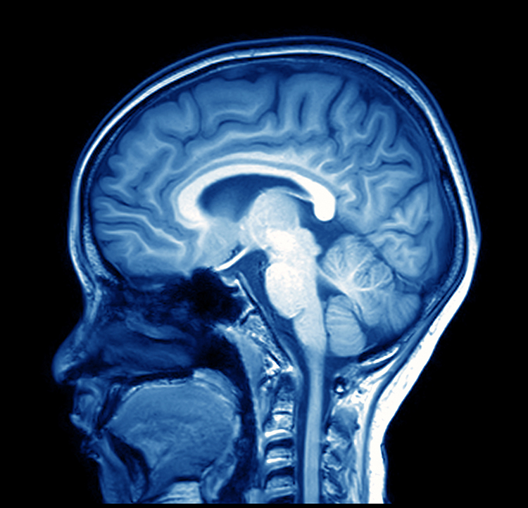
MRI scans' superior spatial resolution can detect demyelination in disorders like multiple sclerosis that CT scans would miss (Breedlove & Watson, 2023). Graphic © MriMan/Shutterstock.com.

FUNCTIONAL TECHNIQUES

Functional techniques reviewed in this section include the EEG and qEEG, magnetoencephalography (MEG), functional magnetic resonance imaging (fMRI), positron emission tomography (PET), and single-photon computerized emission tomography (SPECT). See Lebby (2013) for an excellent overview of these techniques. Also, consult the McGill brain imaging tool module.

EEG

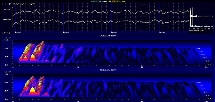
EEG and qEEG can be conceptualized as functional imaging techniques. A single-channel EEG performs “neuroimaging” by displaying an image of microvolts in adjacent 1-Hz bins or adjacent bands (e.g., a 2D spectrogram (shown below) or with a 3D spectrogram. Graphic © John S. Anderson.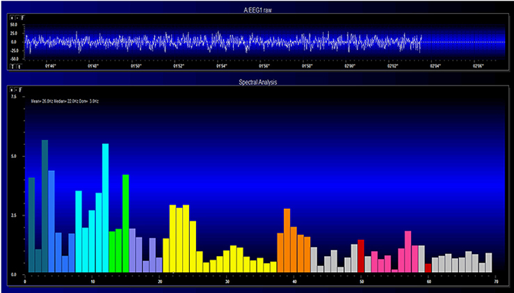






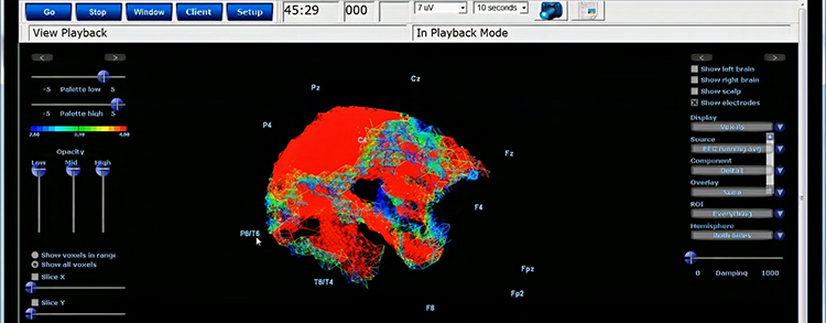
Further, 19-channel qEEG methods show images of activity as it is distributed across the brain’s convexity (i.e., over a 2D 10-20 map) or in 3 dimensions using more advanced qEEG methods (e.g., LORETA). Graphic courtesy of BrainMaster Technologies.

Magnetoencephalography

Magnetoencephalography (MEG) is a noninvasive functional imaging technique that uses SQUIDs (superconducting quantum interference devices) to detect the weak magnetic fields generated by neuronal activity. As with the EEG/qEEG, spatial resolution is inferior (cm compared to mm) to the functional MRI (fMRI) (Breedlove & Watson, 2023).

MEG's millisecond temporal resolution allows it to measure rapidly shifting patterns of cortical circuit activation (Breedlove & Watson, 2023). Researchers may combine MEG with MRI to better delineate the cortical structures generating the magnetic fields (Lin et al., 2004). Magnetoencephalography Graphic © Image Source Trading ltd/Shutterstock.com.

Functional Magnetic Resonance Imaging (fMRI)

Functional Magnetic Resonance Imaging (fMRI) generates intense magnetic fields to indirectly detect brain regions' oxygen use during specific tasks.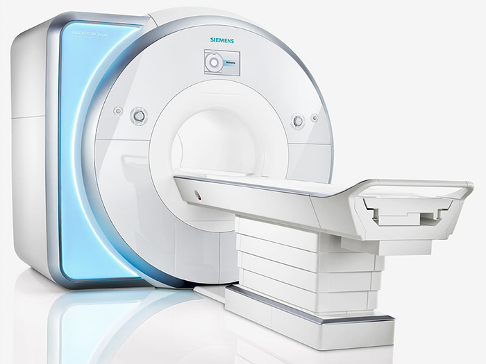




fMRI images represent communications from other neurons and changes in local potentials instead of action potentials. A scanner's magnet strength, measured in teslas (T), directly influences its spatial resolution, which is quantified in terms of voxel size. Higher magnet strength improves the signal-to-noise ratio, allowing for finer spatial resolution and smaller voxel sizes, resulting in more detailed and precise imaging. Advanced research scanners reach 7.0 T.

Although higher spatial resolution in imaging may appear advantageous, it carries the risk of misinterpreting artifacts as functional brain areas. Increased granularity can introduce more noise and potential artifacts, complicating the differentiation between true physiological signals and spurious data. Therefore, achieving an optimal balance between resolution and signal quality is crucial to ensure accurate functional interpretations. A voxel graphic is shown below.




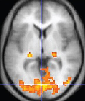
Although the fMRI is limited by significant (100-ms to several-s) delays, it can reveal network contribution to cognitive performance. The fMRI trades spatial resolution for PET's superior temporal resolution (Breedlove & Watson, 2023). A fMRI image © Wikipedia is shown below.

Positron Emission Tomography

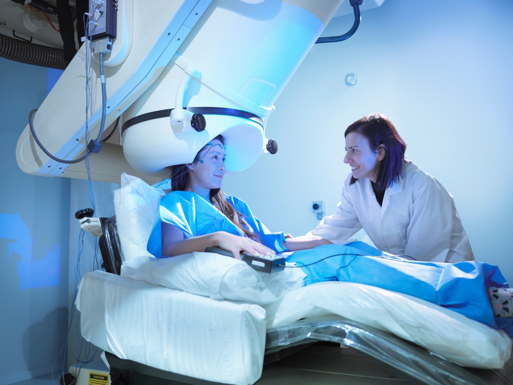
Positron emission tomography (PET) is a functional imaging technique that injects radioactive chemicals into the brain's circulation to measure brain activity (Breedlove & Watson, 2023). PET scan graphic © Gorodenkoff/Shutterstock.com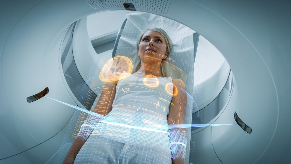





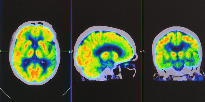
PET scans achieve low temporal resolution (seconds to minutes) with moderate spatial resolution. PET images © Yok_onepiece/Shutterstock.com are shown below.

Single-Photon Emission Computerized Tomography

Single-photon emission computerized tomography (SPECT) is a functional imaging technique that uses gamma rays to create three-dimensional images and slice images of cerebral blood flow averaged over several minutes. Graphic © rumruay/Shutterstock.com.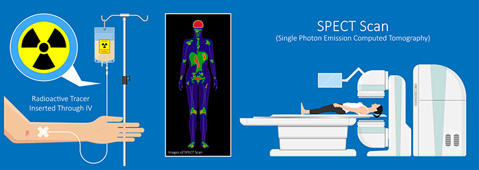




SPECT achieves limited temporal (minutes) and spatial resolution (centimeters).

Using a Limited Number of Electrodes

Peer-reviewed evidence suggests that more EEG channels provide a more accurate assessment and achieve superior clinical or performance outcomes than fewer channels (Lau et al., 2012).

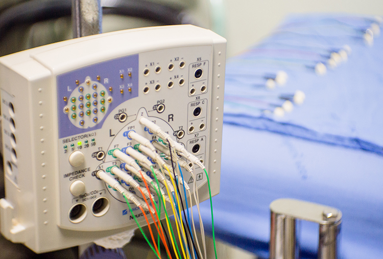
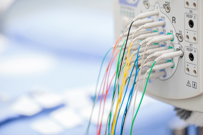
Although some practitioners conduct assessment and training with a single channel, assessments and training methods that use more than one channel have become more available. For example, the cost of a full 19-channel EEG assessment has decreased substantially. Such an assessment can provide not only EEG amplitude data from all sites in the 10-20 system but additionally makes calculations of metrics such as coherence and phase that give information on how well the 10-20 sites communicate with each other. These data from multi-channel methods are beneficial for complex symptom profiles like those associated with Autism Spectrum Disorders, epilepsy, and traumatic brain injury (Thompson & Thompson, 2016). Graphic © Chaikom/Shutterstock.com.




A channel is an EEG amplifier output resulting from scalp electrical activity from three electrode/sensor connections to the scalp. These sensors are commonly known as active, reference, and ground electrodes, though they are more appropriately called positive +, negative - and reference. They are placed on the head in the following manner: an active or positive electrode is placed over a known EEG generator like Cz. A reference or negative electrode may be located on the scalp, earlobe, or mastoid. A ground/reference electrode may also be placed on an earlobe or mastoid (Thompson & Thompson, 2015).

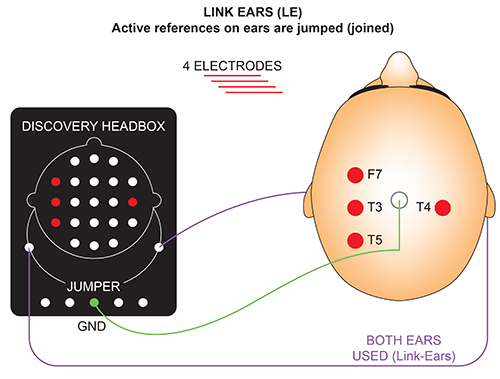
Active and reference sensors are identical balanced inputs and interchangeable. However, some neurofeedback data acquisition systems require the designation of a specific sensor as a "reference," as in a linked-ears reference.

The graphic below was redrawn from John Demos' BCIA-recommended Getting Started with EEG Neurofeedback (2nd ed.). The ear references are connected as a common reference for the four active electrodes (F7, T3, T4, and T5).





A derivation is the assignment of two electrodes to an amplifier's inputs 1 and 2. For example, Fp1 to O2 means that Fp1 is placed in input 1 and O2 in input 2.

A montage groups electrodes together (combines derivations) to record EEG activity (Thomas, 2007).

All montages compare EEG activity between one or more pairs of electrode sites.

Modern amplifiers record all input sensors in reference to a common sensor - often Cz - and all montage (sensor comparison) changes are performed in the software. Amplifiers no longer require manual switching of electrodes between inputs.

The narrated video below © John S. Anderson displays the same 21-channel recording viewed using different montages with a 60-Hz notch filter on and off.

Montage Options and Their Consequences

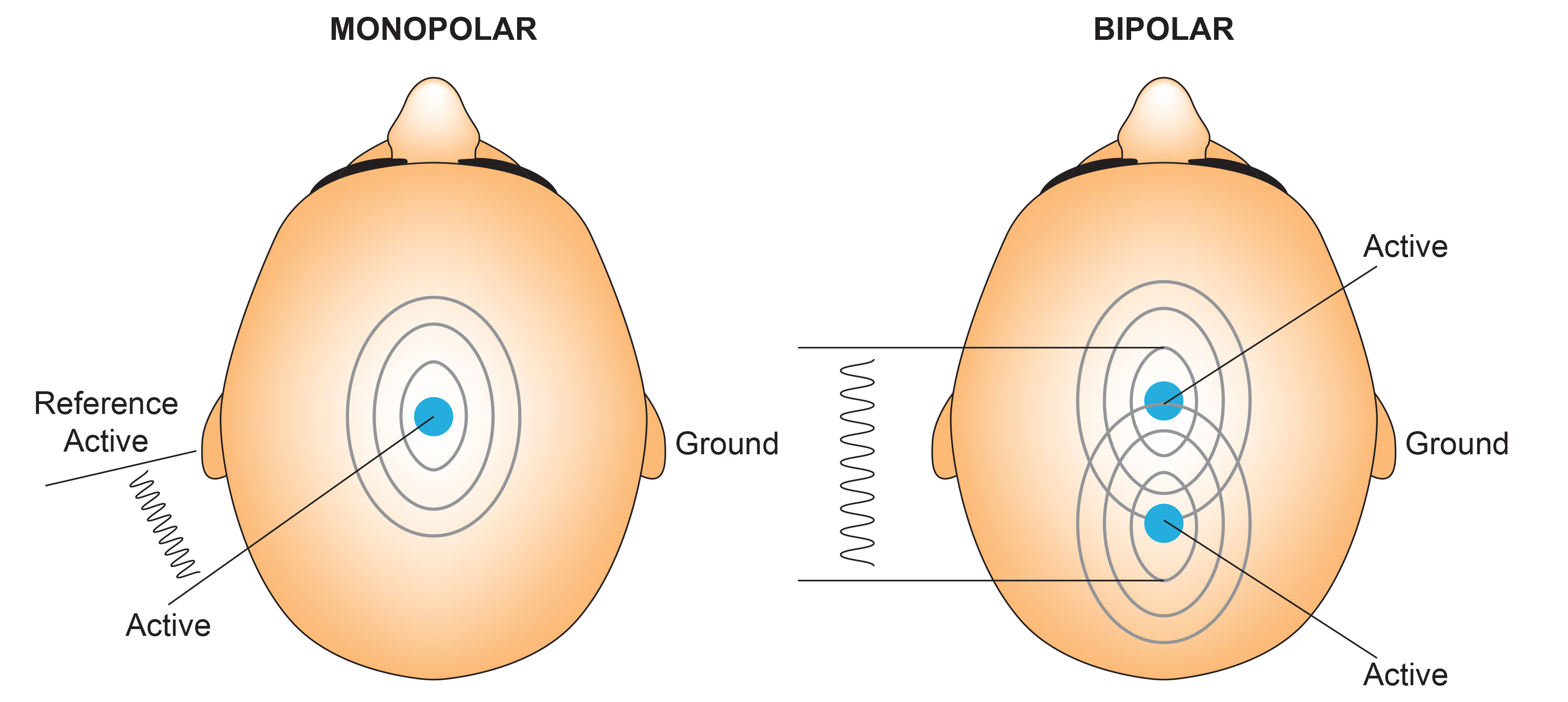
Referential (Monopolar) Montage

A referential (monopolar) montage places one active electrode (A) on the scalp and a "neutral" reference (R) and ground (G) on the ear or mastoid. Graphic adapted by minaanandag on fiverr.com.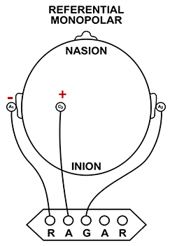




A referential montage assumes that the EEG activity seen on the computer screen represents the active (+) site because the reference (-) site is assumed to be neutral (i.e., producing no EEG activity) and because of the subtraction of signals produced by noise and artifacts that are common to both active and reference sites (common-mode rejection).

The graphics below were redrawn from from John Demos' BCIA-recommended Getting Started with EEG Neurofeedback (2nd ed.). In the right diagram, the active electrode "sees" 7 microvolts while the reference "sees" 0 microvolts, for a total voltage of 7 microvolts.






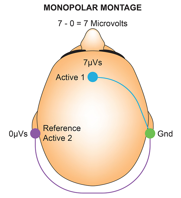
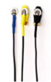
In the photograph below, the blue cable would be used for the active electrode, the yellow cable with an ear clip for reference, and the black cable with an ear clip for the ground.



However, this montage is vulnerable to artifacts from the contraction of facial muscles (Demos, 2019).  The ear reference is also known to produce reference contamination, where EEG signals from this electrode are contributed or added to other electrodes via the mechanism of the differential amplifier, where anything different between the "active" and "reference" sensors is retained. This commonly results in alpha activity produced by posterior alpha sources close to the ear.

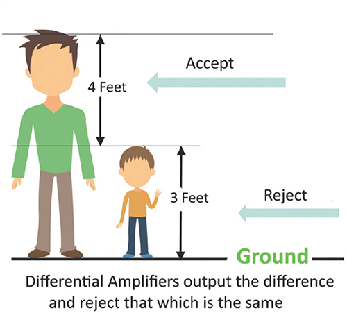
The graphic below was redrawn from John Demos' BCIA-recommended Getting Started with EEG Neurofeedback (2nd ed.). A differential amplifier rejects the common voltage (e.g., 3 feet) and outputs the voltage difference (e.g., 4 feet). A single-ended amplifier outputs the entire voltage (e.g., 7 feet, EEG artifact and signal value).

Sequential (Bipolar) Montage

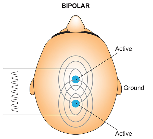
A sequential (bipolar) montage presents a sequence of comparisons of positive (+) and negative (-) electrodes (often called ‘active’ and ‘reference’) that are attached to sites on the scalp and therefore considers the reference electrode to be a second active electrode. The ground (G) electrode is attached to the scalp, to an earlobe, or over the mastoid process. Graphic adapted by minaanandag on fiverr.com.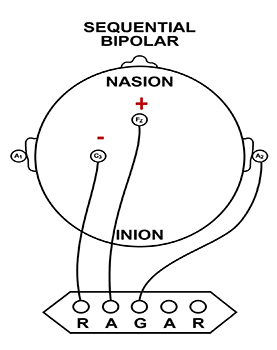




The sequential (bipolar) montage detects the difference in EEG between the positive and the negative electrodes (active and reference), as the referential montage does. Still, now the signal for the channel represents the difference between two sources of EEG activity.

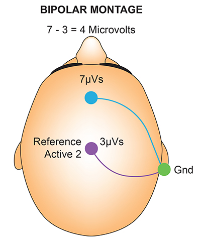
The graphics below were redrawn from from John Demos' BCIA-recommended Getting Started with EEG Neurofeedback (2nd ed.). In the diagram on the right, the active "sees" 7 microvolts while the reference "sees" 3 microvolts. A differential amplifier subtracts these voltages, leaving 4 microvolts.






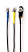
In cases when 19-channels are used, this montage is usually presented with electrode pairs shown in sequence. Note that only the black cable for the ground has an ear clip in the photograph below. 



When used as only a single channel, this montage does not detect localized EEG activity well because it shows only the difference between the A and R signals. However, when used as part of a 19-channel assessment, it localizes EEG events related to epilepsy. This montage can also reduce artifacts when the A and R electrodes are relatively close.

A sequential montage is frequently used in neurofeedback and trains the difference between EEG activity at the A and R electrodes. However, when neurofeedback training produces a change, it remains uncertain whether it is because of a change in EEG at the A electrode, the R electrode, or both electrodes.

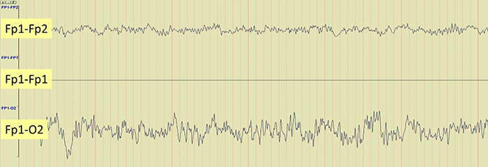
The EEG record appears more similar when sensors are closer together and less similar when they are farther apart (Fp1-O2). When electrodes are spaced close together (Fp1-Fp2), this montage may reject actual EEG activity (Fp1-Fp1). Graphic © John S. Anderson.

Montages for 21 Recording Electrodes

All montages compare EEG activity between one or more pairs of electrode sites.

Please click on the podcast icon below to hear a lecture over the first half of this unit.


The choice of montage does not alter the raw cortical electrical activity itself, but rather filters, enhances, or diminishes aspects of it based on the spatial relationship between electrodes and the dipolar sources within the brain.

A montage defines how each EEG channel is constructed by determining which electrodes are compared to each other. Broadly, montages fall into two categories: bipolar and referential.

In a bipolar montage, each channel represents the voltage difference between two adjacent or anatomically aligned electrodes. This configuration emphasizes local voltage gradients and is especially useful for identifying focal abnormalities, such as epileptiform discharges, through phase reversals—a key diagnostic feature. The longitudinal bipolar montage, also known as the "double banana," arranges channels along the anterior-posterior axis, while the transverse montage organizes them across the coronal plane from left to right. Both are classic examples of bipolar configurations and are commonly employed in clinical EEG for their effectiveness in spatial localization and waveform morphology analysis.

In contrast, a referential montage displays the voltage at each active electrode relative to a common reference point. This reference may be a single electrode, a pair of electrodes, or a mathematically computed value such as the average of all electrodes. Referential montages are particularly suited for assessing global brain activity, hemispheric asymmetries, and background rhythms. Examples include the average reference montage, where each electrode is referenced to the mean of all electrodes; the Cz reference montage, which uses the vertex (Cz) as the fixed reference; and the linked ears montage, which references all electrodes to the average of the earlobes (A1 and A2). The Laplacian montage is a specialized form of referential montage in which each electrode is compared to a weighted average of its immediate neighbors, enhancing the spatial resolution of focal activity.

This section will examine the structure, clinical utility, and interpretive implications of each of these montages. By understanding the fundamental distinction between bipolar and referential configurations—and the strengths and limitations of specific montages within these categories—clinicians can select the most appropriate montage for a given diagnostic question. Furthermore, the ability to apply multiple montages to the same EEG data set, known as re-montaging, enables a more comprehensive and nuanced analysis, ultimately enhancing the accuracy of neurophysiological interpretation in both routine and complex clinical contexts.

Longitudinal Bipolar Montage

The longitudinal bipolar (double banana) montage, is one of the most widely employed configurations in clinical electroencephalography. It consists of a series of bipolar derivations arranged in parallel, linking electrodes from the frontal to the occipital poles along the midline and lateral chains of the scalp. For example, one chain may include the derivations Fp1–F3, F3–C3, C3–P3, and P3–O1, forming a continuous pathway along the left hemisphere. A mirror set is applied on the right: Fp2–F4, F4–C4, C4–P4, and P4–O2. These pairings create an electrical map that is optimal for detecting activity propagating along the anterior-posterior axis of the cerebral cortex.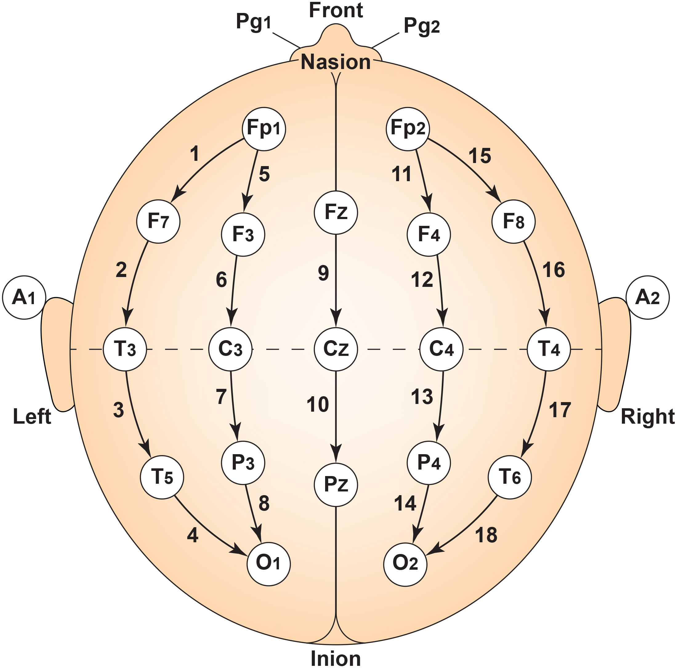

Strengths

The primary strength of this montage lies in its capacity to enhance phase reversals, which are the inversion points of waveform polarity along the bipolar chain and serve as a crucial diagnostic cue for localizing the maximum field of a focal discharge. When a sharp wave or spike occurs in a cortical region sampled between two electrodes, the voltage gradient between them becomes pronounced, resulting in an easily identifiable phase reversal that pinpoints the site of maximal activity. This makes the montage particularly adept at detecting focal epileptiform activity, especially when it is organized along the sagittal plane (Niedermeyer & da Silva, 2005). The montage is also intuitive and standardized, which facilitates inter-reader reliability across clinical institutions.

Limitations

However, the longitudinal bipolar montage is not without limitations. Because each channel is composed of a bipolar derivation, activity that is spatially generalized across adjacent electrode pairs—such as in generalized epileptic discharges or diffuse slowing—may be attenuated or even cancelled out, particularly if it appears in phase across a chain. Additionally, activity that is vertically or obliquely oriented relative to the anteroposterior axis may be poorly resolved due to the montage’s directional bias. Furthermore, the montage may be less sensitive to activity with a deep cortical origin, such as from mesial temporal structures, which may not produce robust potentials at the scalp surface.

Transverse Montage

The transverse (coronal bipolar) montage is an alternative bipolar configuration in which electrodes are linked across the coronal plane of the scalp, from lateral to medial or from one hemisphere to the other. For example, a typical chain might include F7–F3–Fz–F4–F8 across the frontal row, followed by a second chain of T3–C3–Cz–C4–T4 at the central level, and posteriorly T5–P3–Pz–P4–T6, extending through the parietal and temporal regions. These linkages are designed to visualize activity spreading horizontally across the hemispheres or in a left-right configuration.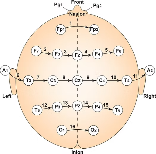

Strengths

The transverse montage is especially advantageous in situations where lateralization is of clinical concern. It is often used as a complementary montage to the longitudinal bipolar in epilepsy workups, as it can delineate whether a waveform or discharge is restricted to one hemisphere, crosses the midline, or is more pronounced on a particular side. By emphasizing horizontal field distribution, the transverse montage improves detection of temporal lobe discharges, which often extend laterally and may appear less prominent in a longitudinal montage. Moreover, the transverse montage is adept at highlighting hemispheric asymmetries in background rhythm and interictal epileptiform activity, offering a different spatial perspective than traditional sagittal derivations.

Limitations

Nonetheless, this montage also presents specific challenges. Its less common use makes it less familiar to many general neurologists, requiring a higher level of interpretive skill and spatial visualization. The absence of anterior-posterior connections can obscure phase reversals along that axis, making it less effective for localizing discharges that originate in midline or parasagittal regions. In addition, the reliance on lateral electrodes introduces greater sensitivity to artifact from facial and temporal muscle activity, which can be a confounding factor in certain recordings.

Average Reference Montage

The average reference montage is conceptually different from bipolar montages in that it is constructed by referencing each active electrode to the mean potential of all scalp electrodes. Mathematically, the signal from each electrode is recalculated as the difference between that electrode and the averaged signal from the full array. The underlying assumption is that the sum of all scalp-recorded potentials approximates zero, creating a neutral reference. In practice, this configuration is implemented in modern digital EEG systems using real-time computational averaging across electrodes, excluding those contaminated by artifact or poor contact. The image below was adapted from Lopez et al. (2017). In most cases, the midline electrodes are also included in these calculations.

Strengths

The primary advantage of the average reference montage is its reference-free nature, which provides a theoretical spatial neutrality. This can be particularly useful in visualizing diffuse, low-amplitude cerebral activity, including generalized spike-wave discharges, slow wave abnormalities, and subtle background fluctuations. Because each electrode is displayed with respect to the same computed reference, spatial comparisons across channels are more direct, making this montage highly valuable in quantitative EEG (qEEG) and source localization studies (Fisch, 1999).

Limitations

However, the montage is also highly susceptible to contamination by a single noisy electrode. If one electrode has a high amplitude artifact (e.g., due to muscle or movement), this can affect the computed average, thereby distorting every channel in the montage. Moreover, the assumption that the average voltage equals zero is only valid when electrodes are evenly distributed and the cortical activity is spatially balanced—conditions rarely met in practice. In the presence of significant focal abnormalities, the average reference can over- or under-estimate the true field of the activity and may even introduce artifactual inversions or misleading asymmetries (Loddenkemper et al., 2014).

Cz Reference Montage

The Cz reference montage is a unipolar configuration in which every scalp electrode is referenced to a single, fixed electrode located at the vertex of the scalp—Cz, the central midline location. This configuration is straightforward and provides consistent spatial orientation for each channel, allowing the reader to compare the amplitude and waveform morphology at different sites relative to a central standard. It is commonly used in event-related potential (ERP) studies, sleep scoring, and pediatric EEG, where ease of interpretation and temporal clarity are prioritized. The image below was adapted from Lopez et al. (2017). In most cases, the midline electrodes are also included in these calculations.

Strengths

One of the key benefits of the Cz reference montage is its ability to reveal lateralized discharges. Because Cz is equidistant from the hemispheres, discharges arising from left or right hemispheres produce strong voltage differences and clear waveforms. The fixed reference also facilitates temporal alignment of discharges, which is useful in assessing spike timing, propagation patterns, and hemispheric synchrony.

Limitations

Nonetheless, Cz is a problematic reference point for activity that originates near the vertex itself, such as discharges from the supplementary motor area, parasagittal cortex, or midline regions. Since the reference is physically close to the source, the recorded potential difference may be minimal or even absent, leading to false negatives. Furthermore, Cz may itself pick up cortical signals, which undermines the assumption of a neutral reference, particularly during periods of midline activation. This limitation becomes particularly relevant when interpreting generalized or midline spike-wave complexes or high-frequency sleep spindles that originate near central sites (Niedermeyer & da Silva, 2005).

Linked Ears Reference (A1-A2 reference or LE) Montage

The linked ears reference montage is a referential EEG configuration in which all scalp electrodes are referenced to a common average of the left and right earlobe electrodes (A1 and A2). These electrodes are presumed to be electrically inactive relative to cerebral sources, providing a stable baseline for assessing cortical activity. In practice, the average of A1 and A2 serves as a reference for each channel, offering a consistent point of comparison across the scalp. This montage has historically been widely used in both routine clinical EEG and intraoperative monitoring due to its simplicity and relatively noise-free reference point (Niedermeyer & da Silva, 2005).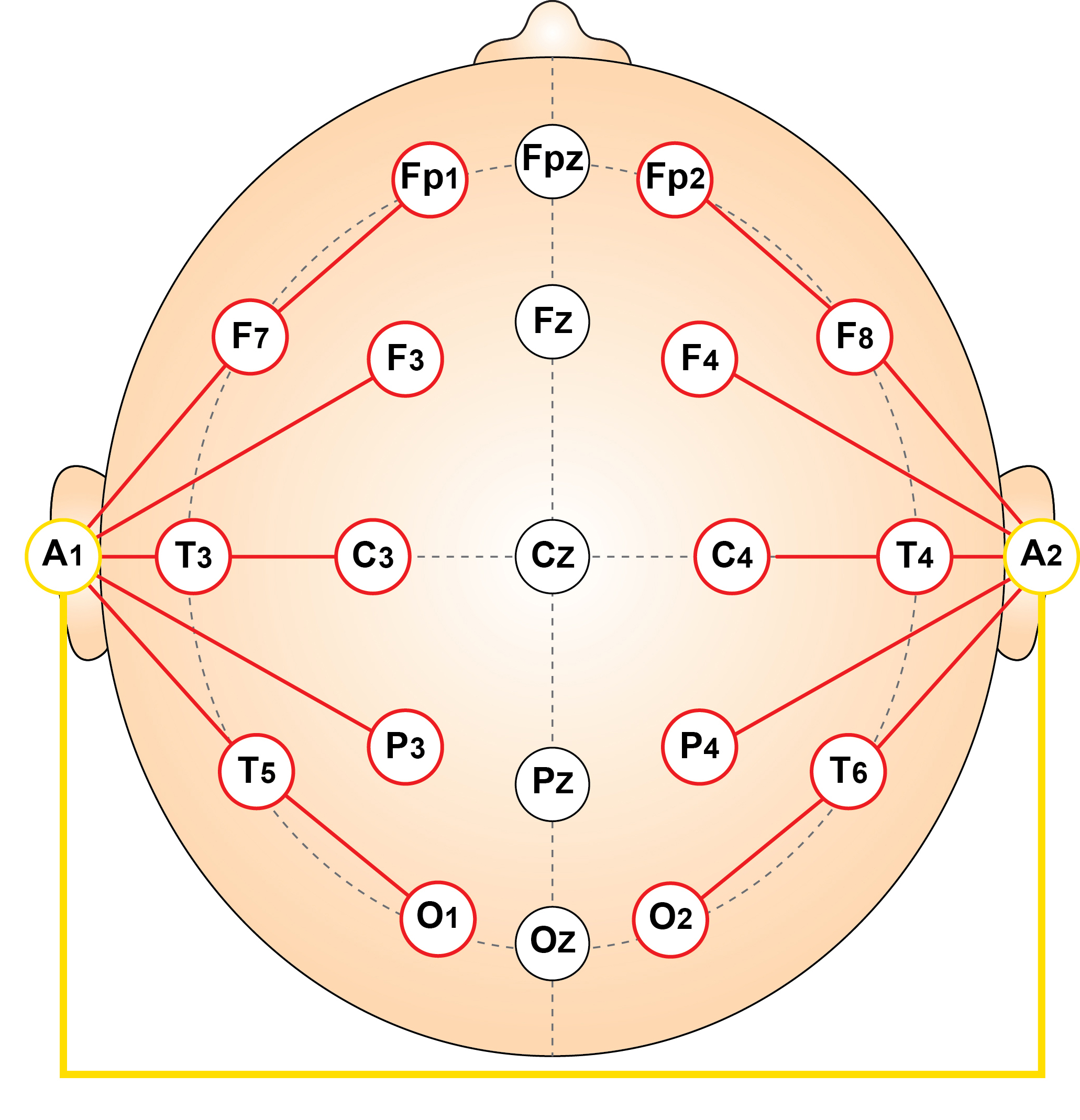

Strengths

The primary strength of the linked ears montage lies in its relative ease of interpretation and its ability to provide clear visualization of regional asymmetries. Because all electrodes are referenced to a common point, focal abnormalities such as interictal epileptiform discharges are often well-demarcated, especially when lateralized. It is also less susceptible to widespread muscle artifacts that may affect central or midline reference points, allowing for improved identification of background rhythms (Nuwer, 1997). Additionally, its long-standing use in clinical practice has made it familiar to many neurologists and EEG technologists, contributing to reproducibility and interpretative consistency.

Limitations

However, the montage is not without limitations. The assumption that the earlobes are electrically inactive is not always valid; in some cases, especially in infants or during high-amplitude discharges, the ears may pick up cortical activity, introducing spurious signals into the reference (Gloor, 1985). Furthermore, asymmetry in earlobe impedance or local artifact can lead to lateralized distortions that mimic or obscure true cerebral asymmetries. The linked ears reference also tends to exaggerate posterior alpha activity and may underrepresent midline or deep sources due to its relatively lateral reference position. As such, while useful in many scenarios, this montage should be interpreted in conjunction with other configurations to ensure accurate localization and characterization of EEG findings.

Laplacian Montage

The Laplacian montage is a type of spatially weighted referential EEG montage designed to enhance the localization of cortical activity by emphasizing signals originating directly beneath each electrode while attenuating those from more distant sources. In this configuration, each electrode is referenced to a weighted average of the surrounding electrodes, thereby approximating the second spatial derivative of the potential field. This mathematical approach enhances local voltage differences and minimizes the effects of broadly distributed or volume-conducted signals. As a result, the Laplacian montage provides improved spatial resolution and is particularly useful in research applications and advanced clinical settings where precise source localization is required (Nunez & Srinivasan, 2006).

Strengths

The Laplacian montage offers significant advantages in localizing focal cortical activity with high spatial precision. Unlike referential montages that rely on ear or mastoid electrodes, the Laplacian configuration excludes these distant references, thereby reducing their influence and minimizing the risk of introducing artifact from electrically active or asymmetrically placed reference sites. Instead, it calculates a spatially weighted average of the surrounding electrodes to serve as the reference for each site, emphasizing the electrical potential directly beneath the electrode of interest. This approach suppresses volume-conducted and broadly distributed signals, allowing for clearer isolation of local cortical activity.

As a result, the Laplacian montage enhances the visibility of subtle, focal EEG features that may be obscured in standard referential or bipolar configurations. It is particularly effective for detecting focal epileptiform discharges, localized slowing, and sensorimotor rhythms, especially when applied in high-density EEG systems where spatial sampling is sufficient to support accurate Laplacian calculations (McFarland et al., 1997). Furthermore, by minimizing global signals and common-mode noise, it offers greater resistance to artifacts from eye movements, muscle activity, and non-neuronal sources such as the diffuse effects of sedative medications or metabolic encephalopathy. These characteristics make the Laplacian montage especially useful in advanced clinical evaluations, functional brain mapping, and neurophysiological research where precise localization is critical. While not typically used as a primary montage in standard EEG interpretation, it serves as a valuable adjunctive tool for refining diagnostic accuracy in complex or ambiguous cases.

Limitations

However, the Laplacian montage also presents notable limitations. Its effectiveness is highly dependent Despite its advantages, the Laplacian montage has important limitations that affect its clinical application. Its accuracy depends on high-density, evenly spaced electrode arrays, making it less reliable in standard low-density systems like the 10–20 montage. A key concern is the edge effect—electrodes at the scalp periphery, such as Fp1, Fp2, F7, F8, O1, and O2, lack surrounding electrodes on all sides, reducing the precision of spatial averaging in these regions. Inadequate electrode coverage can distort rather than enhance localization of cortical signals. Additionally, in some instances, the montage may appear to introduce or redistribute EEG activity, though this is difficult to verify due to the influence of the reference system and signal processing. Furthermore, the spatial filtering inherent to the Laplacian method attenuates slow or widespread activity, limiting its sensitivity to generalized abnormalities such as diffuse slowing or generalized spike-wave discharges (Gordon & Rzempoluck, 2004; Srinivasan et al., 1996). Therefore, while highly effective for focal analysis, the Laplacian montage is best used as a complementary method alongside conventional configurations in clinical EEG interpretation.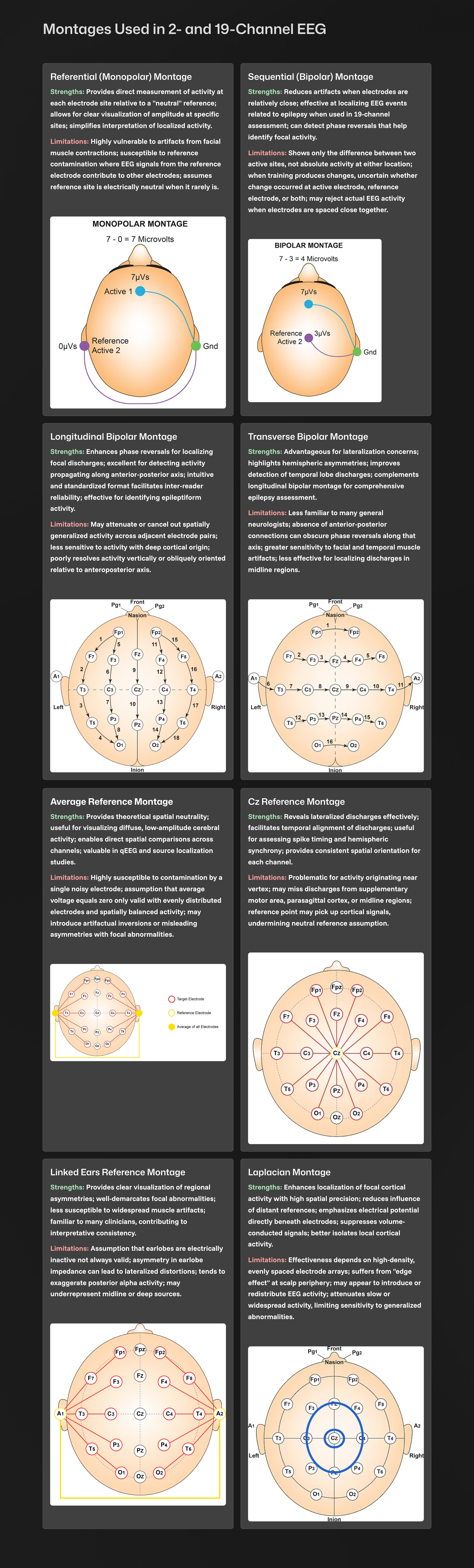

Montage Selection Strategy

Obviously, our goal when viewing the EEG is to identify areas that deviate from typical behavior, correlate those differences with client symptoms, and design a training protocol or group of protocols to address those differences.

The longitudinal bipolar and transverse montages are most effective in demonstrating the key electrographic features of focal abnormalities—namely, clear localization, polarity, and sharp morphology—making them essential in identifying epileptiform discharges and delineating their spatial distribution. The average reference montage, while less sensitive to focal events, contributes significantly to the assessment of hemispheric symmetry and background rhythm integrity, particularly in diffuse or generalized processes. The Cz reference montage provides a reliable lateralized perspective and is especially useful for differentiating left versus right hemispheric activity; however, it lacks optimal resolution for detecting midline sources due to its placement directly over the central vertex.

The linked ears reference montage, commonly used in routine clinical EEG, offers consistency in visualizing lateralized abnormalities and is less susceptible to generalized artifact. However, its reliance on ear electrodes as a common reference introduces potential for asymmetry and contamination, especially in pathological conditions or with poor electrode impedance. In contrast, the Laplacian montage offers superior spatial resolution for identifying focal cortical sources by emphasizing local field potentials and suppressing distant or volume-conducted activity. It is particularly advantageous in high-density EEG systems and functional mapping but requires careful interpretation due to limitations in edge accuracy and reduced sensitivity to generalized abnormalities.

Understanding the comparative strengths and limitations of each montage—bipolar for sharpness and polarity, average reference for symmetry and background, Cz for lateralization, linked ears for routine focal analysis, and Laplacian for high-resolution localization—enables a more nuanced and precise interpretation of EEG findings. This integrative approach enhances diagnostic accuracy and supports informed clinical decision-making in epilepsy evaluation and broader neurophysiological assessment.

Re-Montaging

In clinical electroencephalography, the montage used to display EEG data fundamentally shapes how brain activity is visualized and interpreted. Each montage, whether longitudinal bipolar, transverse, average reference, or Cz reference, has distinct strengths and limitations. However, an essential feature of modern EEG analysis is that clinicians are not limited to a single montage when evaluating an EEG recording. Because digital EEG systems preserve the raw voltage potential at each electrode, clinicians can reconfigure how these signals are displayed by applying different montages to the same epoch of data. This process, known as re-montaging, allows for a more complete and nuanced understanding of the recorded brain activity.

Re-montaging enables clinicians to re-express the same underlying electrical signals in different spatial contexts. A particular waveform or discharge may appear more prominent, localized, or sharply contoured in one montage and more diffuse or less distinct in another. For example, a spike that is clearly localized with a phase reversal in a longitudinal bipolar montage may appear attenuated or blended with surrounding activity in an average reference montage. Conversely, generalized discharges may be more clearly appreciated in referential montages, such as the average or Cz reference, whereas bipolar montages may obscure them due to cancellation effects.

Clinicians re-montage not only to improve visualization of specific events but also to clarify ambiguous findings. A sharply contoured waveform seen in a bipolar montage can be cross-checked in a referential montage to determine whether it reflects true cortical activity or a muscle artifact. Similarly, rhythmic slowing that appears focal in one configuration may prove to be part of a more diffuse process when re-displayed using another montage. This comparative approach helps avoid misinterpretation, particularly in cases where benign variants or technical artifacts could otherwise be mistaken for pathologic activity.

Re-montaging also supports more accurate localization. Some montages are aligned along specific anatomical axes and are therefore more sensitive to discharges propagating in particular directions. The longitudinal bipolar montage, for instance, follows the anterior-posterior axis and is well-suited for identifying phase reversals in that orientation. However, it may not capture lateral propagation across hemispheres as effectively as the transverse montage. By re-montaging into both configurations, a clinician can more precisely triangulate the source of epileptiform discharges or assess whether a waveform is confined to one hemisphere or crosses the midline.

Moreover, the ability to re-montage is indispensable in certain clinical scenarios. When evaluating patients for focal epilepsy, the need to localize seizure onset to a particular lobe or hemisphere is paramount. Re-montaging can reveal subtle asymmetries or focal features that might not be visible in the original display. In cases of suspected encephalopathy, re-montaging into an average reference montage may better demonstrate diffuse slowing or triphasic waves. In sleep EEGs, where vertex sharp waves and sleep spindles may be crucial, the choice of reference becomes especially important, as certain references may suppress or distort these midline phenomena.

Digital EEG systems have made re-montaging straightforward and immediate. Rather than being constrained by the montage selected during acquisition, clinicians can explore different configurations at any point during interpretation. This flexibility is endorsed by the American Clinical Neurophysiology Society, which recommends the use of both bipolar and referential montages and emphasizes the need for clarity, simplicity, and interpretability in montage design. Their guidelines further encourage the use of at least 16 recording channels and the full complement of 10–20 system electrodes to ensure comprehensive spatial sampling and re-montage capability.

Ultimately, the purpose of EEG is to accurately identify and characterize brain activity, whether normal or abnormal, diffuse or focal, transient or rhythmic. No single montage can fully reveal all aspects of this activity. By using multiple montages to re-express the same epoch of EEG, clinicians can compensate for the spatial and referential limitations of individual configurations. This approach allows for the confirmation of findings across montages, facilitates more precise localization, and strengthens diagnostic confidence. The ability to re-montage is not just a technical convenience, it is a critical component of rigorous EEG interpretation and a powerful tool in clinical neurophysiology.

When we identify an EEG feature representing slowed alpha, high amplitude frontal theta activity, excess fast activity, lack of a typical alpha response, or any other finding in one montage, we want to verify and validate that finding using additional montages.

Following the average reference montage, the Laplacian montage can be useful for further zeroing in on the areas of interest.

Finally, the linked ears montage must be consulted if only to identify areas of likely reference contamination that may affect subsequent topographic z-score maps, phase, coherence and network analyses, and other downstream evaluations.

Use Consistent Settings

One important consideration for viewing the EEG is to use consistent settings. The EEG is often viewed using a 50 μV y-scale (vertical axis) and a 30 mm per second x-axis (horizontal) equivalent "chart speed" display.

In the early days of EEG, tracings were drawn by pens suspended over moving chart paper. A typical speed for adult EEG was 30 mm per second and for pediatric EEG was 15 mm per second. Now that almost all EEG is digital, similar equivalent displays show the EEG in this format. This is so the waves appear consistently the same every time they are viewed and can also be compared to reference sources. If different visual display settings are used, then it is difficult to identify wave patterns and abnormally high or low voltage values by visual inspection.

Most modern EEG software uses display time settings indicated in seconds rather than chart speed equivalents. In the NeuroGuide database, the setting that appears most similar to 30 mm per second is 10 seconds per page. Also, in this program, the y-scale setting adjusts automatically depending on the highest voltage present in the recording. It doesn’t allow for a constant setting, though the desired setting can be made manually each time the montage is changed.

Best Practices from the American Clinical Neurophysiology Society Guideline 3 (2016)

The Committee reaffirms the statements pertaining to montages set forth previously in the Guidelines of the American Clinical Neurophysiology Society (ACNS) and that are paraphrased as follows: (a) that no less than 16 channels of simultaneous recording be used, and that a larger number of channels be encouraged,

(b) that the full 21 electrode placements of the 10-20 system be used,

(c) that both bipolar and referential montages be used for clinical interpretation,

(d) that the electrode derivations of each channel be clearly identified at the beginning of each montage,

(e) that the pattern of electrode connections be made as simple as possible, and that montages should be easily comprehended,

(f) that the electrode pairs (bipolar) preferentially should run in straight (unbroken) lines and the interelectrode distances kept equal,,

(g) that tracings from the more anterior electrodes be placed above those from the more posterior electrodes on the recording page, and,

(h) that it is very desirable to have some of the montages comparable for all EEG laboratories.,

2.2 The Committee recommends a “left above right” order of derivations, i.e., on the recording page, left-sided leads should be placed above right-sided leads for either alternating pairs of derivations or blocks of derivations. This recommendation coincides with the prevailing practice of most EEG laboratories, at least in North America and in many other areas.

Recognizing and Correcting Signals of Noncerebral Origin

EEG artifacts, consisting of noncerebral electrical activity, can be divided into physiological and exogenous artifacts. Physiological artifacts include electromyographic, electro-ocular (eye blink and eye movement), cardiac (pulse), sweat (skin impedance), drowsiness, and evoked potential. Exogenous artifacts include movement, 60 Hz and field effect, and electrode (impedance, bridging, and electrode pop) artifacts.

Please click on the podcast icon below to hear a lecture over the first half of this unit.




The movie features a 19-channel BioTrace+ /NeXus-32 display of EEG artifacts © Mary Tracy.

Electromyographic (EMG) Artifact

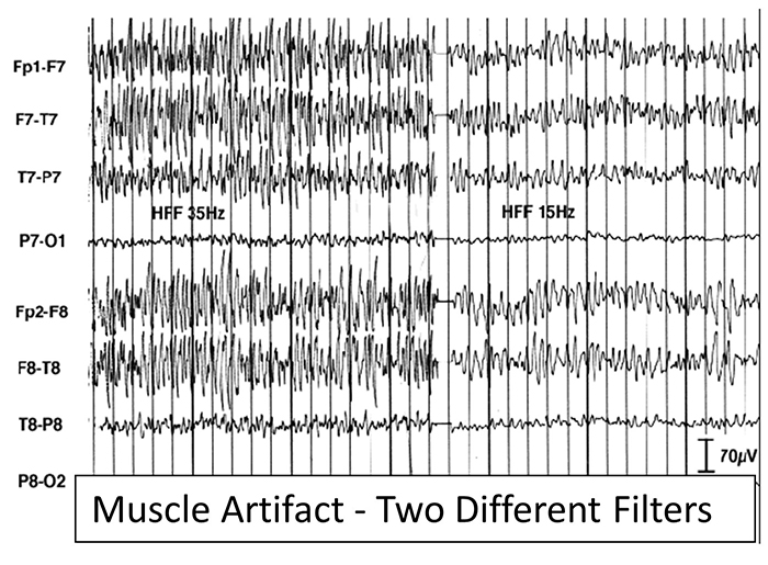
EMG artifact is interference in EEG recording by volume-conducted signals from skeletal muscles.

This artifact contains high-frequency activity that resembles a "buzz" of fast activity during a contraction. EMG is seen as fast beta activity in the qEEG. While some frequencies are between 10-70 Hz, most are 70 Hz or higher.

The graphic shows how high-frequency filter (HFF) selection can affect contamination by this artifact. A high-frequency filter (low-pass filter) attenuates frequencies above a cutoff frequency. In the examples below, the cutoffs are 35 Hz and 15 Hz.

All the channels on the left side of the tracing show SEMG artifact admitted by a 35-Hz high-frequency filter. The right tracing is free from SEMG artifact since its 15-Hz high-frequency filter attenuates the higher frequencies that contain this artifact.



The next graphic shows how gum chewing can generate SEMG artifact by contracting the muscles of mastication. Graphics © eegatlas-online.com.




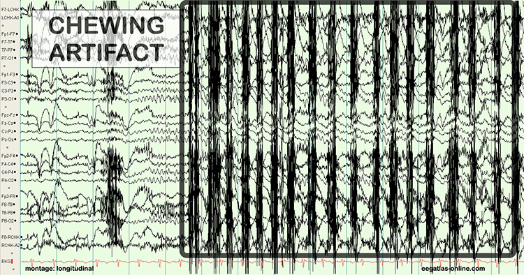
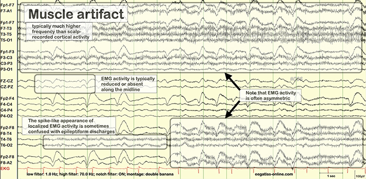
The frequency spectrum for SEMG artifact ranges from 2-1,000 Hz. While strong muscular contraction can contaminate all frequency bands, including 10 Hz, the beta rhythm (at 70 Hz or higher) is most affected by this artifact. EMG artifact may create the appearance of greater beta activity than is present. Graphic © eegatlas-online.com.




Below is a BioGraph ® Infiniti EMG artifact display. Note how the amplitude of the EEG spectrum increases with each contraction.





Thompson and Thompson (2016) observed that EMG artifact is readily detected because it affects one or two channels, particularly at T3 and T4 at the periphery, and less often at O1, O2, Fp1, and Fp2.

You can identify EMG artifact by visually inspecting the raw signal. The next graphic shows SEMG artifact using a 70-Hz high-frequency filter.

Electro-Ocular Artifact

Electro-ocular artifact contaminates EEG recordings with potentials generated by eye blinks, eye flutter, and other eye movements. For example, anxious patient eyelid flutter may cause deflections at Fp1 and Fp2 (Klass, 2008).

This artifact is due to the movement of the eye’s electrical field when the eye rotates and the contraction of the extraocular muscles. The eye creates a dipole that is electropositive at the front and electronegative at the back. Bell’s Phenomenon refers to the upward rotation of the eye when it closes and causes an artifact seen as an apparent increase in EEG.

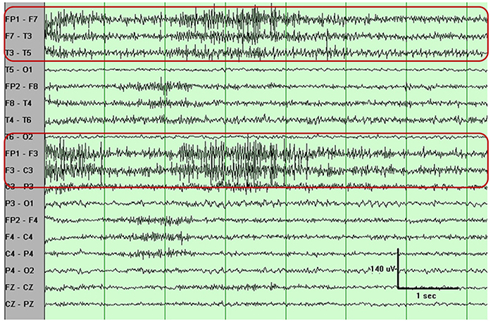
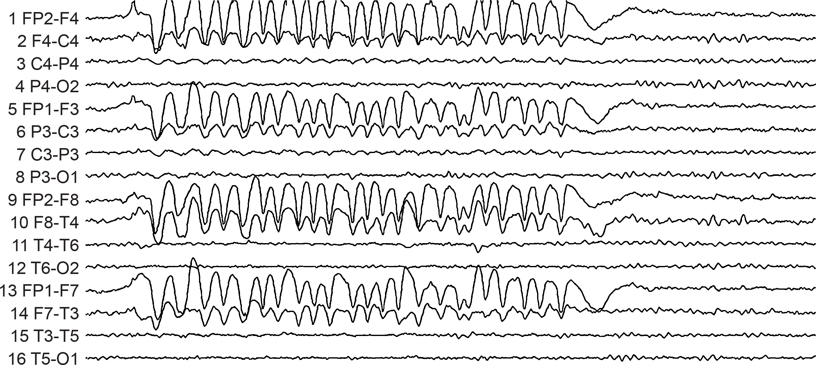
Both eye artifacts can mimic meaningful EEG patterns, particularly to the untrained eye, thus affecting assessment results, most notably when utilizing normative database comparisons. Lateral eye movements during an eyes closed recording can appear as delta activity because they generally fall within that 1-4 Hz frequency band. Blink artifact can look like sharp spike and wave patterns associated with seizure activity, particularly when repetitive, such as with eye flutter.

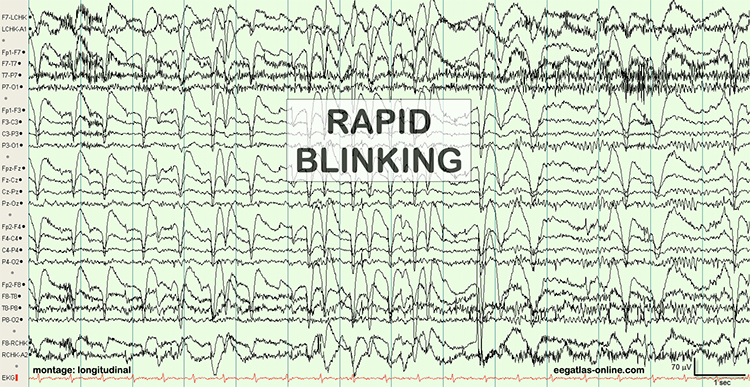
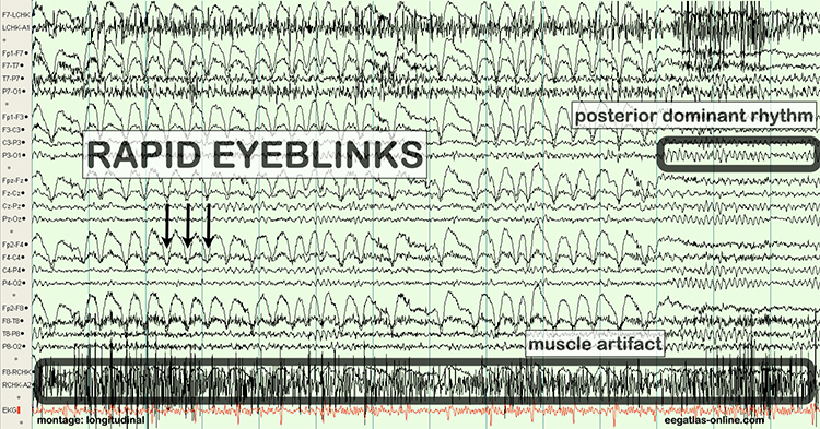
The next two graphics show eye movement artifacts due to rapid blinking. Graphics © eegatlas-online.com.







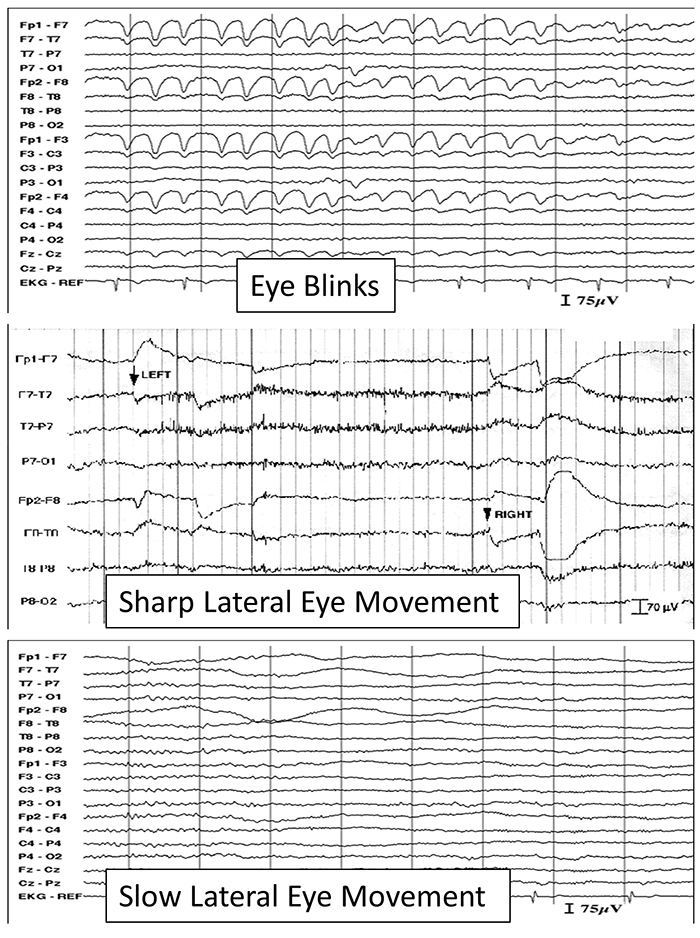
The next graphic shows eye blinks, sharp lateral eye movement, and slow lateral eye movement.




Below is a BioGraph ® Infiniti EEG display of eye movement artifact.





Below is a NeXus display of eye blink and EMG © John S. Anderson.




An upward eye movement will create a positive deflection at Fp1, while a downward eye movement may create a negative deflection. In a longitudinal sequential montage, the artifact is typically seen at frontal sites (Fp1- F3 and Fp2-F4). A left movement may produce a positive deflection at F7 and a negative deflection at F8 (Thompson & Thompson, 2015).

Rapid eye flutter may resemble seizure activity. Graphic redrawn by minaanandag on fiverr.com.

Cardiac and Pulse Artifacts

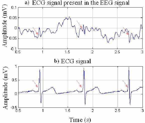
Cardiac artifact occurs when the ECG signal appears in the EEG (Jiang et al., 2019). This artifact may be produced when electrode impedance is imbalanced or too high or when an ear electrode contacts the neck. The frequency range for ECG artifact is 0.05-80 Hz, and it contaminates the delta through beta bands. Since multiple electrodes detect this artifact, it can create the appearance of greater coherence than is present. Graphic © eegatlas-online.com.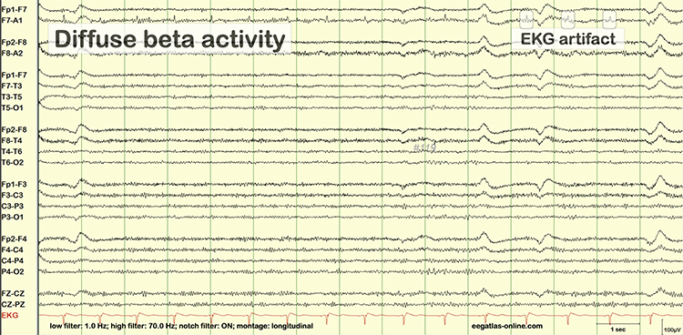




You can detect cardiac artifacts by inspecting chart recorder, data acquisition, or oscilloscope displays of the raw EEG waveform. Cardiac artifact appears as a wave that repeats about once per second (Thompson & Thompson, 2016). Below is a BioGraph ® Infiniti ECG artifact display.


 


ECG artifacts are easily recognized, especially when there is a separate ECG tracing, allowing a direct comparison between recorded ECG and artifact in the EEG. Sharp, regular and consistent artifacts at about 1 per second in the EEG are likely the result of the ECG. The artifact is observed best in referential montages using earlobe electrodes A1 and A2 or mastoid electrodes M1 and M2 and any such patterns in the EEG that are synchronous with the ECG tracing can be identified as such an artifact. ECG artifact graphic was produced by Garces et al. (2007).





Another cardiac-related artifact are the pulse artifacts that occur when an EEG electrode is placed directly over a blood vessel. The mechanical movement of the electrode as a vessel expands and contracts will produce a slow-wave pattern in the EEG that can be mistaken for delta activity and will affect topographic maps created from data containing such an artifact. This is sometimes called the cardioballistic artifact though another similar looking artifact is thought to be related to the subtle movement of the body as the heart beats. Graphic © eegatlas-online.com.




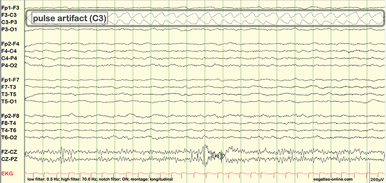
ECG and pulse artifact appear in topographic EEG maps as delta frequency activity, leading to false positive findings related to excess delta.

Sweat (Impedance) Artifact

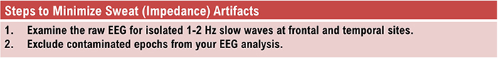
Sweat artifact results from sweat on the skin changing the conductive properties under and near the electrode sites (i.e., bridging artifact). Sweating reduces electrode contact with the scalp and generates large-scale up and down EEG line movements in several frontal channels. This artifact is often elicited by abrupt, unexpected stimuli and usually appears as isolated 1-2 Hz slow waves of 1-2-s duration at frontal and temporal sites (Thompson & Thompson, 2015). Graphic © eegatlas-online.com.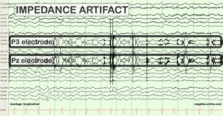

Bridging Artifact

A short circuit produces bridging artifact between adjacent electrodes due to excessive application of electrode paste/gel or a client who is sweating excessively or who arrives with a wet scalp. Bridging artifacts can cause adjacent electrodes to create a short circuit that produces identical referential EEG recordings or a flat line with a bipolar montage. The Fp1-F3 channel's reduced amplitude and frequency illustrate a bridging artifact.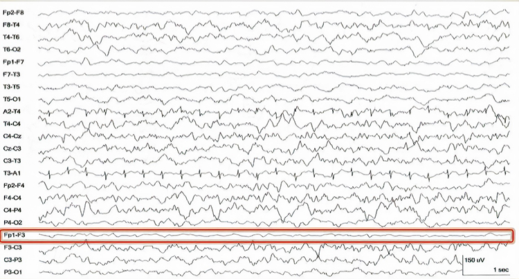

Drowsiness Artifact

Drowsiness artifact is the appearance of stage 1 or stage 2 sleep in the EEG. Stage 1 and stage 2 of sleep are most likely during eyes-closed recording. Sleep may occur during eye-closed awake recording. Graphic © eegatlas-online.com.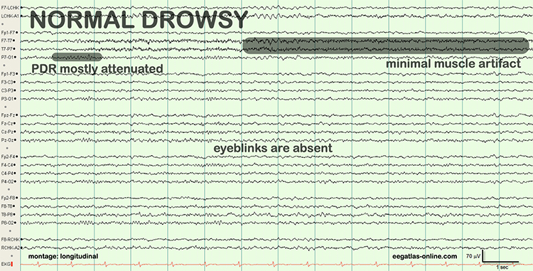




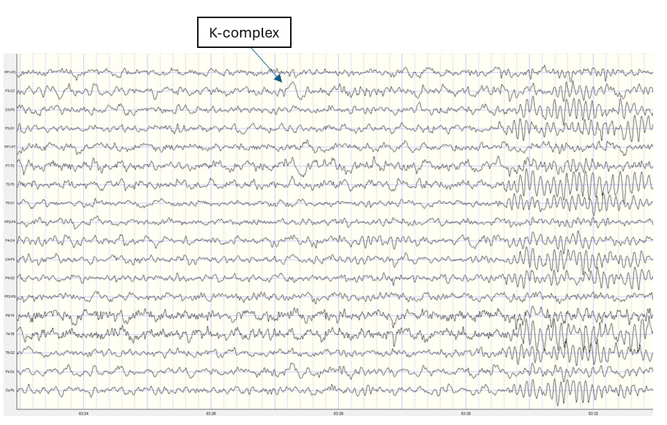
Two additional drowsiness artifact examples appear below. The first shows a brief episode of drowsiness lasting about 5 seconds with a dropout of the alpha rhythm (posterior dominant rhythm - PDR) and then a return of the PDR. The second example shows the end of a longer period of light sleep with a K-complex indicated in the F3-C3 derivation, followed by a return to a typical alpha rhythm.





Stage 1 sleep is a subtle drowsy state which clients often do not recognize. Alpha amplitude (especially occipital) may markedly decrease, and/or theta (especially frontal) may increase. Reductions in EMG and beta amplitude will accompany slow eye-rolling movements. Sleepiness may be accompanied by spike-like transients (vertex or V-waves). The graphic below © John S. Anderson shows increased theta during stage 1 sleep.





When you detect drowsiness artifact during a training session, suspend recording and instruct your clients to move their hands and legs to increase wakefulness. To avoid this artifact, ask them to retire early and sleep for 9 hours if possible (Thompson & Thompson, 2003).

Evoked Potential

Evoked potential artifact (also called event-related potential artifact) consists of somatosensory, auditory, and visual signal processing-related transients that may contaminate multiple channels of an EEG record. While evoked potentials increase recording variability and reduce its reliability, they minimally affect averaged data (Thompson & Thompson, 2015).

Watch BPM Biosignals' YouTube video EEG: Visually evoked potentials (VEP).

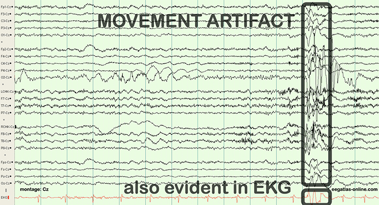
Movement Artifact

Movement artifact is caused by client movement or the movement of electrode wires by other individuals. Most of these artifacts are produced by brief changes in electrode-skin surface connection. Cable movement is called cable sway.

Movement artifacts can produce high-frequency and high-amplitude voltages identical to EEG and EMG signals. While the delta rhythm is most affected by this artifact, it may also contaminate the theta band (Thompson & Thompson, 2016). Graphic © eegatlas-online.com.




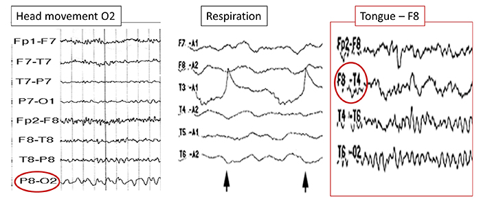
The graphic below shows movement artifacts due to head movement (left), respiration (center), and tongue movement (right).



Below is a BioGraph ® Infiniti cable movement artifact display. Note the two voltage spikes at the beginning of the recording.

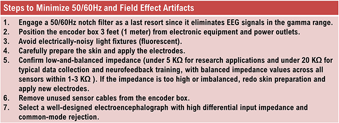
50/60 Hz and Field Artifacts

Both 50/60 Hz and field artifacts are external artifacts transmitted by nearby electrical sources. For example, power adapters for laptop computers or other electronic devices are common sources for this type of artifact.

While 60-Hz artifact is a risk in North America where AC voltage is transmitted at 60 Hz, 50-Hz artifact is a problem in other locations that generate power at 50 Hz. Their fundamental frequency is 50 or 60 Hz with harmonics at 100/120 Hz, 150/180 Hz, and 200/240 Hz.

Unfortunately, subharmonics of 50/60 Hz signals may remain in the EEG, even when notch filters are used, resulting in ½ or ¼ frequency signals contaminating the actual neural signals at approximately 25 Hz and 12.5 Hz (for 50-Hz artifact) or 30 Hz and at 15 Hz (for 60 Hz artifact).

Imbalanced electrode impedances increase an EEG amplifier's vulnerability to these artifacts. The 60-Hz artifact graphic below © John S. Anderson.




A BioGraph ® Infiniti display of 60-Hz artifact is shown below in red. Note the cyclical voltage fluctuations and 60-Hz peak in the power spectral display.

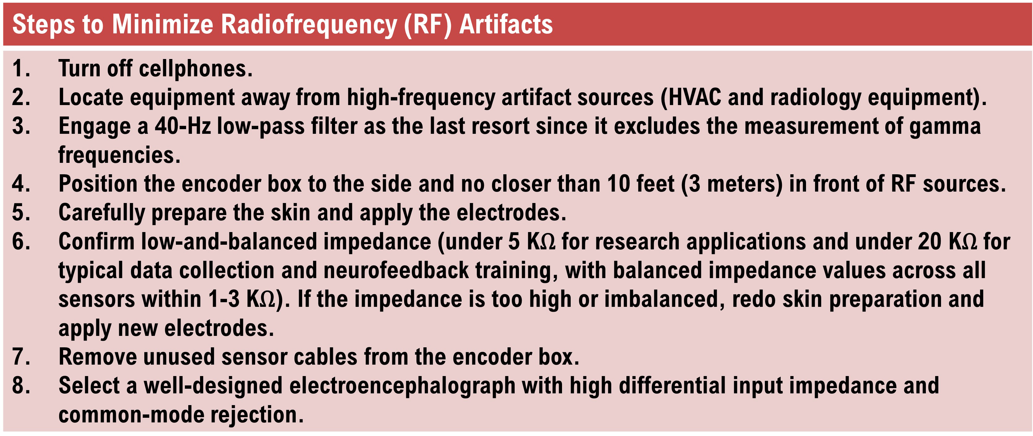
Radiofrequency Artifact

Radiofrequency (RF) artifact radiates outward like a cone from the front of televisions and computer monitors. Graphic © eegatlas-online.com.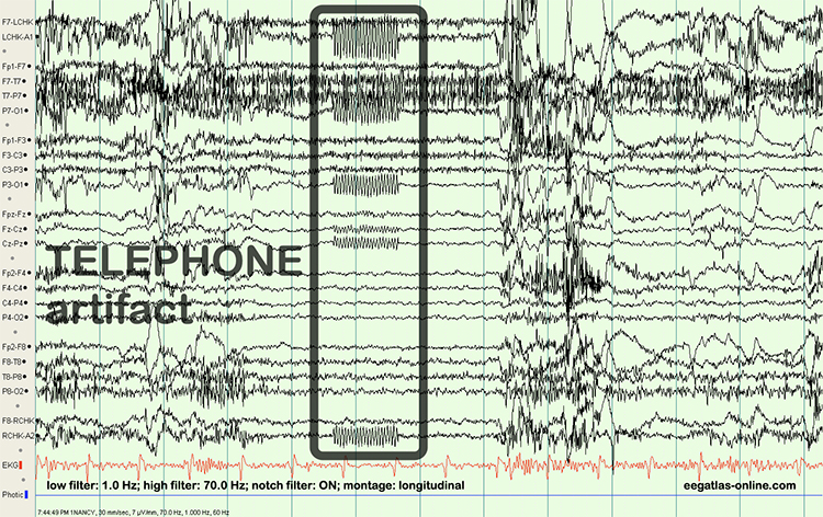

Electrode Artifacts

There are several sources of electrode artifacts. Even with proper care, electrode surfaces can become corroded and the leads and connectors damaged. Using sensors with mismatched electrode metals can cause polarization of amplifier input stages.  

Impedance Artifact

Unless skin-electrode impedance is low (under 5 KΩ for research and 20 KΩ for training) and balanced (under 1-3 KΩ ), diverse artifacts like 50/60 Hz and movement can contaminate the EEG signal, as seen in the P3 and Pz electrodes. Graphic © eegatlas-online.com.





Regular impedance checks during setup ensure consistent contact quality. Using abrasive gels or prepping the skin to reduce impedance is crucial, particularly in long-duration studies where skin conditions may change over time.

However, infection control procedures must be enhanced whenever electrode attachment methods breach intact skin, due to the risk of disease transmission from bodily fluids. Modern, high input impedance amplifiers have nearly eliminated the need for these more invasive methods, even in sensitive recordings.

Electrode Pop Artifact

Even when the impedance is low and balanced, mechanical disturbance (e.g., bubbles or voids) can produce a unique artifact. Electrode pop artifact has a sudden large deflection in at least one channel when an electrode abruptly detaches from the scalp. This may also happen when there is a bubble or other defect in the gel or paste, and a charge builds up and subsequently "jumps" across the gap, resulting in a large electrical discharge. Graphic © John S. Anderson.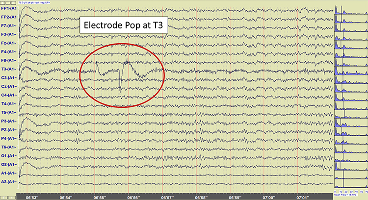

Recognizing Normal EEG Patterns

This section covers normal EEG patterns, including the posterior dominant rhythm, differences between eyes open and eyes-closed resting conditions, developmental aspects of the EEG, and diurnal influences on the EEG.

Normal EEG Patterns

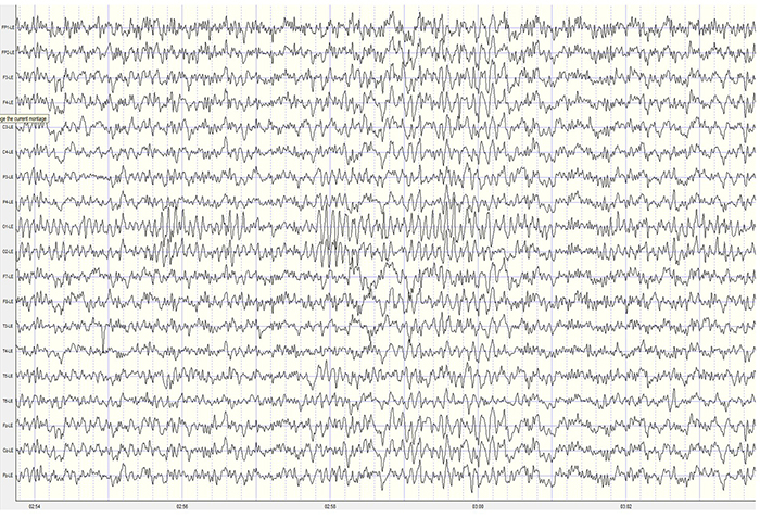
The healthy adult EEG is a cerebral symphony comprised of theta, alpha, sensorimotor rhythm, beta, and gamma activity. We will survey the generators, distributions, and behavioral correlates of these rhythms. EEG rhythms correlate with patterns of behavior (level of attentiveness, sleeping, waking, seizures, and coma), occur in distinct frequency ranges, and are characterized by synchrony and desynchrony.

Synchrony means that pools of neurons coordinate their firing due to pacemakers (left) and mutual coordination (right). Synchrony graphic redrawn from Bear, Connors, and Paradiso (2002) by minaanandag at Fiverr.com.





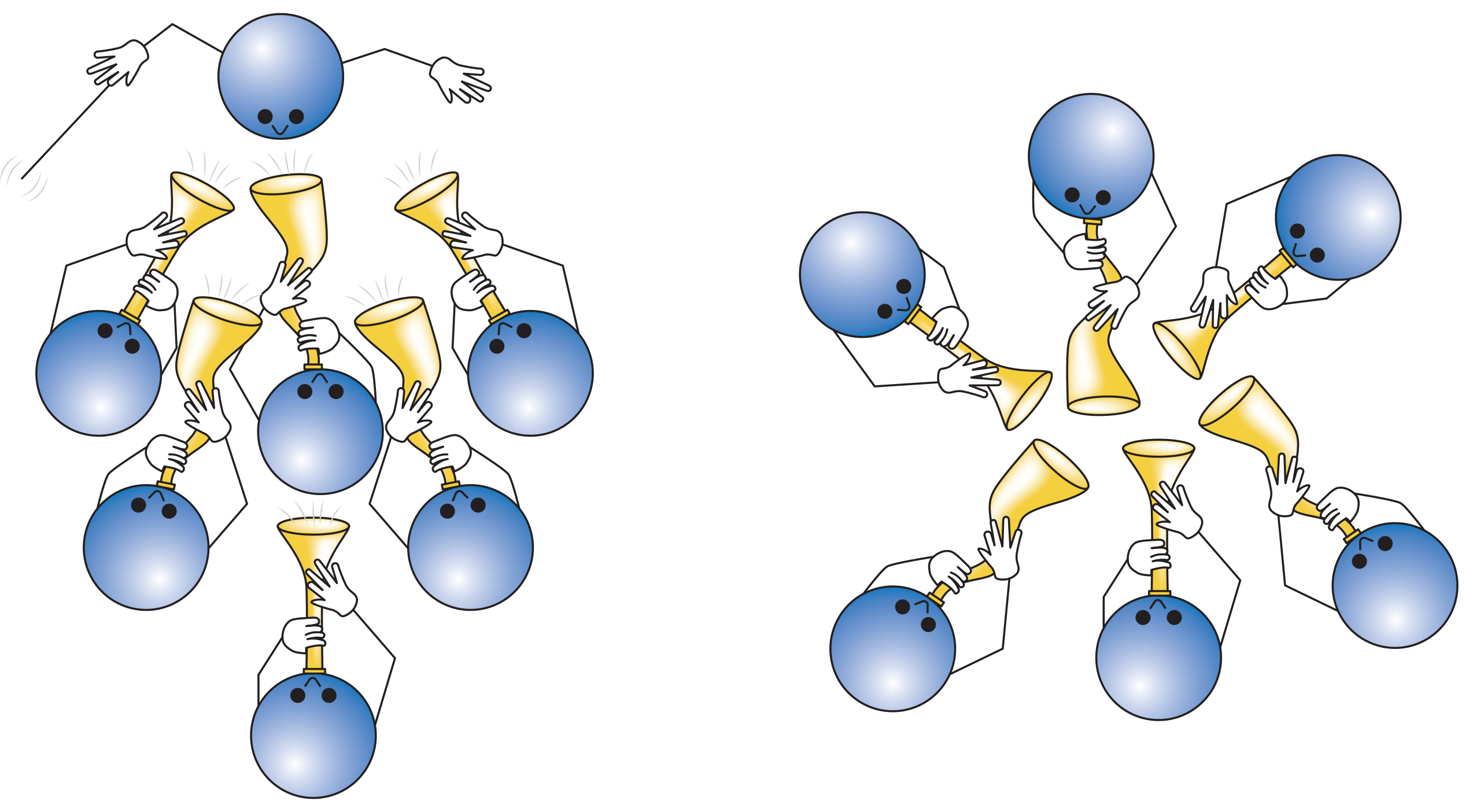
The synchronized EEG graphic below © John S. Anderson.




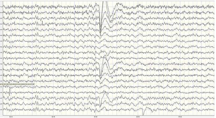
Desynchrony means that pools of neurons fire independently due to stimulation of specific sensory pathways up to the midbrain and high-frequency stimulation of the reticular formation and nonspecific thalamic projection nuclei.

The desynchronized EEG graphic below © John S. Anderson.






Graphic © John S. Anderson.

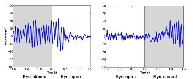
Effect of Eyes Open and Closed Conditions on the EEG

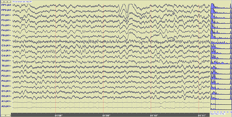
The alpha rhythm is strongly modulated by visual input. Opening the eyes blocks or reduces the occipital alpha rhythm. Hans Berger (1929) originally described this phenomenon. In contrast, eyes-closed alpha is associated with alert wakefulness and reduced visual input (Thompson & Thompson, 2016).

The movie below is a 19-channel BioTrace+ /NeXus-32 display of eyes open and closed EEG © John S. Anderson. Note the appearance of alpha activity with eyes closed at about 14 seconds and alpha-blocking with eyes open at about 45 seconds.




The graphic below illustrates alpha-blocking and was uploaded to ResearchGate by the author, Byoung-Kyong Min. The two trials show alpha-blocking during eyes-open conditions.

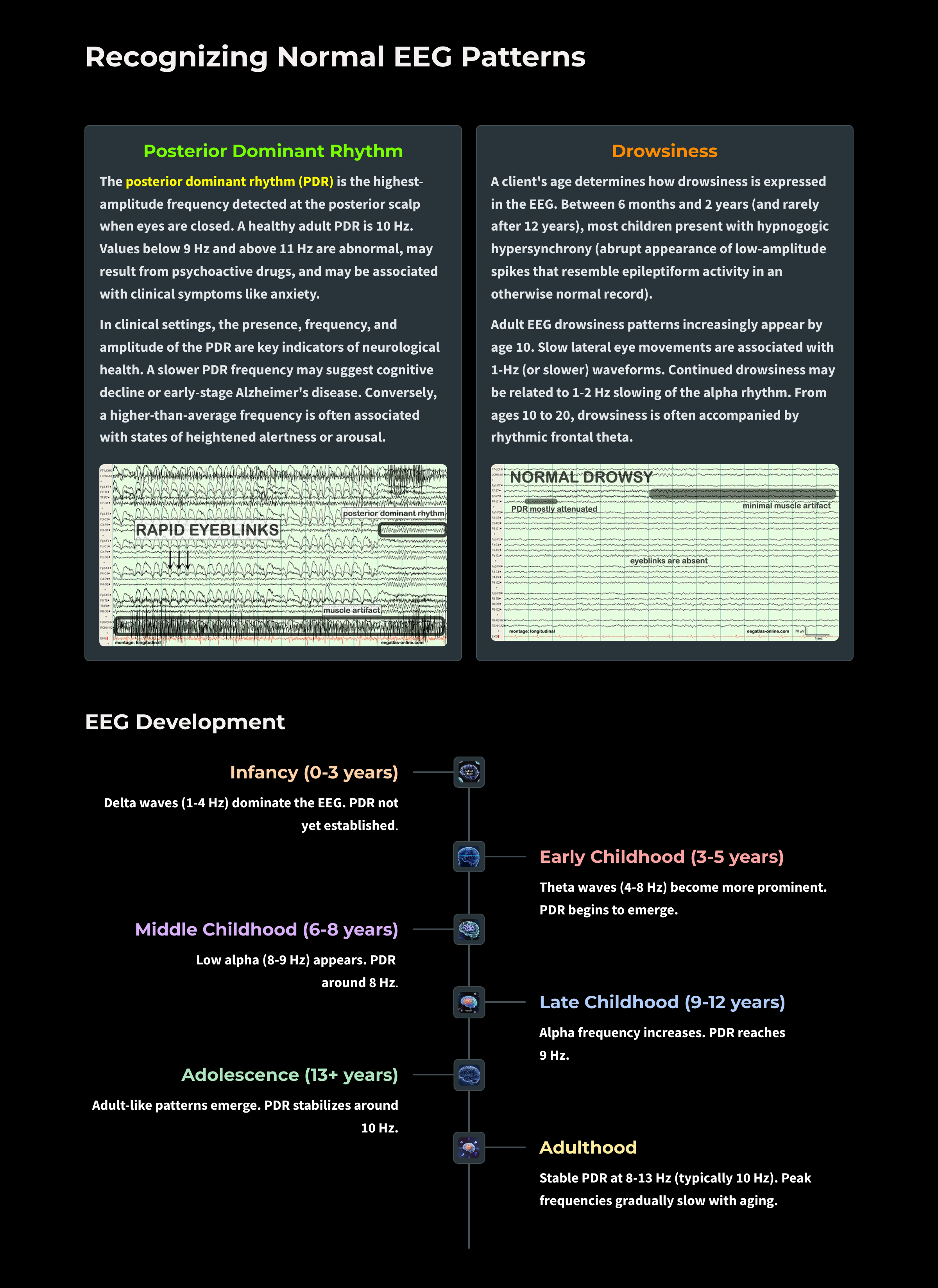
Posterior Dominant Rhythm

The posterior dominant rhythm (PDR) is the highest-amplitude frequency detected at the posterior scalp when eyes are closed. A healthy adult PDR is 10 Hz. Values below 9 Hz and above 11 Hz are abnormal, may result from psychoactive drugs, and may be associated with clinical symptoms like anxiety (Demos, 2019).

In clinical settings, the presence, frequency, and amplitude of the PDR are key indicators of neurological health. A slower PDR frequency, for example, may suggest cognitive decline or early-stage Alzheimer’s disease. Conversely, a higher-than-average frequency is often associated with states of heightened alertness or arousal. The symmetry of the PDR across hemispheres is another important consideration, as significant asymmetry may indicate structural abnormalities, such as a stroke, tumor, or impact-related traumatic brain injury.

Graphic © eegatlas-online.com. See the PDR at P3-O1.

Developmental Aspects of EEG

Delta is dominant below age 3, theta from 3 to 5, and low alpha from 6 to 8. Alpha frequency increases to a peak around 10 Hz after age 10. The transition from infancy to childhood is marked by the development of alpha rhythms, particularly in the posterior regions. The alpha frequency increases with age, starting at around 6 Hz in early childhood and reaching the adult range of 8-13 Hz by adolescence. This progression mirrors the maturation of thalamocortical circuits, which play a key role in generating rhythmic activity.

These changes and the ones that follow reflect the increasing differentiation of the cortex and sub-cortical structures, increases in longer distance network connections and enhanced communication between the differentiated structures as each area of the brain begins to specialize to process and/or integrate neural functions such as sensory input and executive tasks.

Peak frequencies slow during adulthood with aging (Thompson & Thompson, 2016). The PDR rises with age: 1 year (6 Hz), 8 years (8 Hz), 10-12 years (9 Hz), and 13-14 years (10 Hz) (Demos, 2019).

Diurnal Influences on the EEG

Alpha and theta rhythm amplitudes vary across the day, with the highest values at 11 am, 1 pm, and 3 pm. Fatigue and individual differences (but not eating) influence the magnitude of change and precise peak times. Serial assessments should be conducted at the same time of day to control for diurnal fluctuations (Thompson & Thompson, 2015).

Evaluation of Subject Variables During Acquisition

Subject variables are crucial to the interpretation of EEG measurements. In this section, we will examine the importance of alertness-drowsiness, physical relaxation, and anxiety. We covered the effects of eyes closed/eyes open in the previous section and medication effects in the Psychopharmacology unit. As a reminder, medications like benzodiazepines, which enhance inhibitory neurotransmission, tend to increase the amplitude of the PDR. Stimulants like caffeine can reduce its presence. Understanding these pharmacological effects is crucial for interpreting EEG results in patients on medication.

Alertness-Drowsiness

A client's age determines how drowsiness is expressed in the EEG. Between 6 months and 2 years (and rarely after 12 years), most children present with hypnogogic hypersynchrony (abrupt appearance of low-amplitude spikes that resemble epileptiform activity otherwise normal record). Beta activity between 20-25 Hz also maximally appears centrally and posteriorly. When older children and adults are drowsy or enter stage 1 and 2 sleep, frontocentral beta may be activated (Fisch, 1999).

Adult EEG drowsiness patterns increasingly appear by age 10. Slow lateral eye movements are associated with 1-Hz (or slower) waveforms that can be detected with the greatest amplitude and reverse polarity at F7 and F8. Continued drowsiness may be related to 1-2 Hz slowing of the alpha rhythm. For this reason, it is crucial to confirm client wakefulness when assessing alpha rhythm frequency (Fisch, 1999. Graphic © fizkes/Shutterstock.com.



From ages 10 to 20, drowsiness is often accompanied by rhythmic frontal theta (Fisch, 1999).

Physical Relaxation

The human stress response is multidimensional and involves diverse systems, ranging from the central nervous system to the immune system. Each person uniquely responds to stressors. This is called response stereotypy.

Individuals differ in which systems are involved, the degree of their activation or suppression, and the impact of these changes on their health.

Since clients show widely different response stereotypies, assessment should monitor multiple physiological channels, including blood volume pulse (BVP) for heart rate and heart rate variability, electromyography (EMG), a respirometer for respiration rate and pattern, skin conductance (SC), and skin temperature.

A capnometer, which measures end-tidal CO2, can complement the information provided by a respirometer by detecting CO2 reductions due to overbreathing, which is more subtle than hyperventilation (Khazan, 2019).

Professionals can find the normative values for these measures in Moss and Shaffer's (2019) Physiological Recording Technology in Biofeedback and Neurofeedback.

Stress responses that affect physiologic responses outside the CNS can cause artifacts in EEG recordings. Therefore, when client distress produces excessive artifact, a professional may have to coach the client to relax guided by one or more biofeedback modalities.

Clients should be monitored in a comfortable but upright position.

Anxiety

Anxious clients often present with decreased alpha and increased 19-21 Hz or 20-23 Hz beta activity. Conversely, anxious adults diagnosed with ADHD may show increased alpha activity. Even without perceptible sweating, anxious patients may present with intermittent biphasic slow-wave activity (Picton & Hillyard, 1972). Graphic © Peshkova/Shutterstock.com.





Clients who experience panic may exhibit paroxysmal EEG activity (Thompson & Thompson, 2015).

Glossary

50/60 Hz: external artifacts transmitted by nearby electrical sources.

active electrode: an electrode placed over a site that is a known EEG generator like Cz.

alpha-blocking: the replacement of the alpha rhythm by low-amplitude desynchronized beta activity during movement, attention, mental effort like complex problem-solving, and visual processing.

amplitude: the strength of the EEG signal measured in microvolt or picowatts.

artifact: false signals like 50/60Hz noise produced by line current.

asynchronous waves: neurons depolarize and hyperpolarize independently.

average reference montage: an EEG referencing technique where each electrode is referenced to the arithmetic mean of all scalp electrode potentials; used to highlight focal activity and reduce common signals.

bipolar montage: a montage in which each EEG channel represents the voltage difference between two adjacent scalp electrodes.

bridging artifact: a short circuit between adjacent electrodes due to excessive application of electrode paste or a client who is sweating excessively or who arrives with a wet scalp.

cardiac artifact: the contamination of the EEG by the ECG signal.

channel: an EEG amplifier output that is the result of scalp electrical activity from three electrode/sensor connections to the scalp.

computerized axial tomography (CAT or CT): the creation of medium-resolution images of brain structure by moving an x-ray source along an arc surrounding the head.

Cz: the central midline electrode in the 10–20 system, often used as a common reference point in unipolar montages.

derivation: the assignment of two electrodes to an amplifier's inputs 1 and 2.

desynchrony: pools of neurons fire independently due to stimulation of specific sensory pathways up to the midbrain and high-frequency stimulation of the reticular formation and nonspecific thalamic projection nuclei.

differential amplifier (balanced amplifier): a device that boosts the difference between two inputs: the active (input 1) and reference (input 2).

dipolar sources: brain-generated electrical fields that produce opposing voltages detectable at the scalp; critical in EEG localization.

drowsiness artifact: in adults, 1-Hz (or slower) waveforms can be detected with greatest amplitude and reverse polarity at F7 and F8 may progress to 1-2 Hz slowing of the alpha rhythm.

EEG artifacts: noncerebral electrical activity in an EEG recording can be divided into physiological and exogenous artifacts.

electro-ocular artifact: contamination of EEG recordings by potentials generated by eye blinks, eye flutter, and eye movements.

electrode: a specialized conductor that converts biological signals like the EEG into currents of electrons.

electrode pop artifact: sudden large deflections in at least one channel when an electrode abruptly detaches from the scalp.

EMG artifact: interference in EEG recording by volume-conducted signals from skeletal muscles.

epoch: a time segment of EEG recording, usually lasting a few seconds, used to examine waveform characteristics within a specific interval.

evoked potential artifact (event-related potential artifact): somatosensory, auditory, and visual signal processing-related transients that may contaminate multiple channels of an EEG record.

exogenous artifacts: noncerebral electrical activity generated by movement, 50/60 Hz and field effect, bridging, and electrode (electrode “pop" and impedance) artifacts.

field artifacts: external artifacts transmitted by nearby electrical sources.

focal activity: EEG signals that originate from a localized area of the brain, as opposed to generalized activity.

frequency (Hz): the number of complete cycles that an AC signal completes in a second, usually expressed in hertz.

functional magnetic resonance imaging (fMRI): an imaging technique to detect brain regions' oxygen use during specific tasks indirectly.

ground electrode: a sensor placed on an earlobe, mastoid bone, or the scalp that is grounded to the amplifier.

hertz (Hz): unit of frequency measured in cycles per second.

high-frequency filter (HFF): a filter that attenuates frequencies above a cutoff frequency.

hypnogogic hypersynchrony: the abrupt appearance of low-amplitude spikes that resembles epileptiform activity in an otherwise normal record.

impedance (Z): the complex opposition to an AC signal measured in Kohms.

impedance meter: device that uses an AC signal to measure impedance in an electric circuit, such as between active and reference electrodes.

impedance test: automated or manual measurement of skin-electrode impedance.

inion: the bony prominence on the back of the skull.

International 10-10 system: a modified combinatorial system for electrode placement that expands the 10-20 system to 75 electrode sites to increase EEG spatial resolution and improve detection of localized evoked potentials.

International 10-20 system: a standardized procedure for placing 21 recording and one ground electrode on adults.

Laplacian montage: a referential EEG configuration in which each electrode is referenced to a weighted average of its immediately surrounding electrodes. This enhances local cortical activity while suppressing distant or volume-conducted signals, improving spatial resolution for source localization.

linked ears reference montage: a referential EEG configuration in which all scalp electrodes are referenced to the average of the left (A1) and right (A2) earlobe electrodes. This setup assumes the earlobes are electrically neutral and provides a common reference point for assessing cortical activity.

localization: the process of determining the origin of EEG activity within the brain, often aided by montage selection and waveform characteristics.

longitudinal bipolar montage: a bipolar montage where electrodes are connected front-to-back along the anterior-posterior axis; also known as the "double banana" montage.

magnetoencephalography (MEG): a noninvasive functional imaging technique that uses SQUIDs (superconducting quantum interference devices) to detect the weak magnetic fields generated by neuronal activity.

magnetic resonance imaging (MRI): a noninvasive imaging technique that uses strong magnetic fields and bursts of RF energy to construct highly detailed images of the living brain.

mastoid bone: the bony prominence behind the ear.

microvolt (μV): the unit of amplitude (signal strength) that is one-millionth of a volt.

monopolar recording: a recording method that uses one active and one reference electrode.

montage: a grouping of electrodes (combining derivations) to record EEG activity.

motor unit: an alpha motor neuron and the skeletal muscle fibers it innervates.

movement artifact: voltages caused by client movement or the movement of electrode wires by other individuals.

nasion: the depression at the bridge of the nose.

notch filter: a filter that suppresses a narrow band of frequencies, such as those produce by line current at 50/60Hz.

ohm (Ω): the unit of impedance or resistance.

phase reversal: a change in polarity between adjacent electrodes in a bipolar montage, indicating the likely location of maximal voltage and aiding in source localization.

physiological artifacts: noncerebral electrical activity that includes electromyographic, electro-ocular (eye blink and eye movement), cardiac (pulse), sweat (skin impedance), drowsiness, and evoked potential.

polarity: the direction of waveform deflection (positive or negative) in EEG, relevant for determining the source and direction of electrical activity.

polarization: chemical reactions produce separate regions of positive and negative charge where an electrode and electrolyte make contact, reducing ion exchange.

positron emission tomography (PET): a functional imaging technique that injects radioactive chemicals into the brain's circulation to measure brain activity.

posterior dominant rhythm (PDR): the highest-amplitude frequency detected at the posterior scalp when eyes are closed.

preauricular point: the slight depression located in front of the ear and above the earlobe.

pulse artifacts: noncerebral voltages due to mechanical movement of an electrode in relation to the skin surface due to the pressure wave of each heartbeat.

Quantitative EEG (qEEG): digitized statistical brain mapping using at least a 19-channel montage to measure EEG amplitude within specific frequency bins.

reference electrode: an electrode placed on the scalp, earlobe, or mastoid.

referential (monopolar) montage: the placement of one active electrode (A) on the scalp and a neutral reference (R) and ground (G) on the ear or mastoid.

re-montaging: the process of re-displaying EEG data using a different montage configuration, allowing clinicians to view the same recorded electrical activity from alternative spatial perspectives to enhance interpretation, localization, and artifact differentiation.

response stereotypy: a person’s unique response pattern to stressors of identical intensity.

sequential (bipolar) montage: placement of active (A) and reference (R) sensors on active scalp sites and the ground (G) to an earlobe or mastoid.

single photon emission computerized tomography (SPECT): a functional imaging technique that uses gamma rays to create three-dimensional and slice images of cerebral blood flow averaged over several minutes.

spatial resolution: the ability of an EEG montage to distinguish electrical activity arising from different areas of the brain.

sweat artifact: changes in the EEG signal when sweat on the skin changes the conductive properties under and near the electrode sites (i.e., bridging artifact).

synchrony: the coordinated firing of pools of neurons due to pacemakers and mutual coordination.

tragus: the flap at the opening of the ear.

transverse montage: a bipolar EEG montage that links electrodes horizontally across the head, providing sensitivity to lateralized and horizontal propagation of activity.

vertex (Cz): the intersection of imaginary lines drawn from the nasion to inion and between the two preauricular points in the International 10-10 and 10-20 systems.

voxel: a three-dimensional pixel representing a specific volume of brain tissue, used to measure and analyze brain activity and structure.

TEST YOURSELF ON CLASSMARKER

Click on the ClassMarker logo below to take a 10-question exam over this entire unit.

REVIEW FLASHCARDS ON QUIZLET

Click on the Quizlet logo to review our chapter flashcards.

Visit the BioSource Software Website

BioSource Software offers Physiological Psychology, which satisfies BCIA's Physiological Psychology requirement, and Neurofeedback100, which provides extensive multiple-choice testing over the Biofeedback Blueprint.

Assignment

Now that you have completed this module, explain why low-and-balanced skin-electrode impedances are important in neurofeedback training. Describe the precautions you take to achieve acceptable impedance values. How do you measure impedance with your neurofeedback system?

References

Acharya, J. N., Hani, A. J., Thirumala, P. D., & Tsuchida, T. N. (2016). American Clinical Neurophysiology Society Guideline 3: A Proposal for Standard Montages to Be Used in Clinical EEG. Journal of Clinical Neurophysiology: Official Publication of the American Electroencephalographic Society, 33(4), 312–316. https://doi.org/10.1097/WNP.0000000000000317

Andreassi, J. L. (2000). Psychophysiology: Human behavior and physiological response. Lawrence Erlbaum and Associates, Inc.

Basmajian, J. V. (Ed.). (1989). Biofeedback: Principles and practice for clinicians. Williams & Wilkins.

Breedlove, S. M., & Watson, N. V. (2023). Behavioral neuroscience (10th ed.). Sinauer Associates, Inc.

Cacioppo, J. T., & Tassinary, L. G. (Eds.). (1990). Principles of psychophysiology. Cambridge University Press.

Carvalhaes, C., & Acacio de Barros, J. (2014). The surface Laplacian technique in EEG: Theory and methods. International Journal of Psychophysiology, 97(3), 174–188. Collura, T. F. (2014). Technical foundations of neurofeedback. Taylor & Francis.

Demos, J. N. (2019). Getting started with neurofeedback (2nd ed.). W. W. Norton & Company.

Fisch, B. J. (1999). Fisch and Spehlmann's EEG primer (3rd ed.). Elsevier.

Floyd, T. L. (1987). Electronics fundamentals: Circuits, devices, and applications. Columbus: Merrill Publishing Company.

Garces, A., Laciar, E,, Patiño, H., & Valentinuzzi, M. (2007). Artifact removal from EEG signals using adaptive filters in cascade. Journal of Physics: Conference Series, 90(1), 012081. https://10.1088/1742-6596/90/1/012081

Gloor, P. (1985). EEG analysis and the localization of epileptic foci. In D. Daly & T. Pedley (Eds.), Current practice of clinical electroencephalography (pp. 139–174). Raven Press.Gordon, E., & Rzempoluck, E. (2004). Clinical EEG and neuroscience, 35(2), 57–68.

Grant, A. (2015). Four elements earn permanent seats on the periodic table. Science News.

Halford, J. J., Sabau, D., Drislane, F. W., Tsuchida, T. N., & Sinha, S. R. (2016). American Clinical Society Guideline 4: Recording clinical EEG on digital media. Journal of Clinical Neurophysiology, 33(4), 317-319. https://doi.org/10.1080/21646821.2016.1245563

Hugdahl, K. (1995). Psychophysiology: The mind-body perspective. Harvard University Press.

Hughes, J. R. (1994). EEG in clinical practice (2nd ed.). Butterworth-Heinemann.

Khazan, I. Z. (2019). Biofeedback and mindfulness in everyday life: Practical solutions for improving your health and performance. W. W. Norton & Company.

Klass, D. W. (2008). The continuing challenge of artifacts in the EEG. EEG artifacts. American Society of Electroneurodiagnostic Technologists, Inc. https://doi.org/10.1080/00029238.1995.11080524

Kubala, T. (2009). Electricity 1: Devices, circuits, and materials (9th ed.). Cengage Learning.

Lau, T. M., Gwin, J. T., & Ferris, D. P. (2012). How many electrodes are really needed for EEG-based mobile brain imaging? Journal of Behavioral and Brain Science, 2(3), 387-393. https://doi.org/10.4236/jbbs.2012.23044

Lebby, P. C. (2013). Brain imaging: A guide for clinicians. Oxford University Press.

Libenson, M. H. (2010). Practical approach to electroencephalography. Saunders Elsevier.

Lin, F., Witzel, T., Hamalainen, M. S., Dale, A. M., Belliveau, J. W., & Stufflebeam, S. M. (2004). Spectral spatiotemporal imaging of cortical oscillations and interactions in the human brain. NeuroImage, 2(3), 582-595. https://dx.doi.org/10.1016%2Fj.neuroimage.2004.04.027

López, S., Gross, A., Yang, S., Golmohammadi, M., Obeid, I., & Picone, J. (2016). An analysis of two common reference points for EEGs. IEEE Signal Processing in Medicine and Biology Symposium, 2016, https://doi.org/10.1109/SPMB.2016.7846854

McFarland, D. J., McCane, L. M., David, S. V., & Wolpaw, J. R. (1997). Spatial filter selection for EEG-based communication. Electroencephalography and Clinical Neurophysiology, 103(3), 386–394. https://doi.org/10.1016/S0013-4694(97)00022-2

Nuwer, M. R. (1997). Assessment of digital EEG, quantitative EEG, and EEG brain mapping. Report of the American Academy of Neurology and the American Clinical Neurophysiology Society. Neurology, 49(1), 277–292. PMID: 9222191.

Montgomery, D. (2004). Introduction to biofeedback. Module 3: Psychophysiological recording. Association for Applied Psychophysiology and Biofeedback.
 
Niedermeyer, E., & da Silva, F. L. (2005). Electroencephalography: Basic principles, clinical applications, and related fields (5th ed.). Lippincott Williams & Wilkins.

Nilsson, J. W., & Riedel, S. A. (2008). Electric circuits (8th ed.). Pearson Prentice-Hall.

Nunez, P. L., & Srinivasan, R. (2006). Electric fields of the brain: The neurophysics of EEG (2nd ed.). Oxford University Press. 580.2004.12104.x

Peek, C. J. (2016). A primer of traditional biofeedback instrumentation. In M. S. Schwartz, & F. Andrasik (Eds.). (2016). Biofeedback: A practitioner's guide (4th ed.). The Guilford Press.

Picton, T. W., & Hillyard, S. A. (1972). Cephalic skin potentials in electroencephalography. Encephalogr Clin Neurophysiol, 33, 419-424. https://doi.org/10.1016/0013-4694(72)90122-8

Pfister, H., Kaynig, V., Botha, C. P., Bruckner, S., Dercksen, V., & Hege, H.-C. (2012). Visualization in connectomics. Mathematics and Visualization, 37. https://doi.org/10.1007/978-1-4471-6497-5_21

Srinivasan, R., Nunez, P. L., & Silberstein, R. B. (1996). Spatial filtering and neocortical dynamics: Estimates of EEG coherence. IEEE Transactions on Biomedical Engineering, 43(7), 683–693. https://doi.org/10.1109/10.502603

Stern, R. M., Ray, W. J., & Quigley, K. S. (2001). Psychophysiological recording (2nd ed.). Oxford University Press.

Thomas, C. (2007). What is a montage? EEG instrumentation. American Society of Electroneurodiagnostic Technologists, Inc.

Thompson, M., & Thompson, L. (2015). The biofeedback book: An introduction to basic concepts in applied psychophysiology (2nd ed.). Association for Applied Psychophysiology and Biofeedback.