Artifacting

HRV recordings are vulnerable to diverse artifacts that can produce interbeat interval (IBI) values that are too long or too short. The IBI, also called the NN (normal-to-normal) interval when artifacts have been removed, represents the time between consecutive R-spikes in the ECG waveform. Artifacts are false values produced by the client's body (ectopic beats), the client's actions (movement), the environment (line current), and hardware limitations (light leakage).

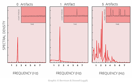
The clinical stakes are high: a single artifactual IBI value in a 2-minute epoch can markedly distort time-domain indices like SDNN, the standard deviation of normal-to-normal intervals (Berntson et al., 1997). This sensitivity to outliers (i.e., extreme values) makes artifact detection and correction essential for valid HRV assessment. Consider that SDNN reflects overall autonomic function—a distorted value could lead you to overestimate or underestimate your client's regulatory capacity.

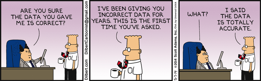
Client assessment and training are only as good as your data. As the familiar saying goes, "garbage in, garbage out." This principle applies whether you are working with a veteran managing PTSD symptoms, an athlete optimizing performance, or a cardiac rehabilitation patient rebuilding autonomic resilience.

We recommend the "close the barn door before the horse escapes" strategy to ensure data integrity. Prevent artifacts before you record data so that you don't have to remove them later. This proactive approach—proper sensor placement, controlled recording conditions, and client preparation—saves time and produces more reliable results than even the most sophisticated correction algorithms. Please review our BVP Hardware and ECG Hardware units for a review of artifacts and strategies to mitigate them.

Manually inspect the raw signal and IBI values to ensure that artifacts do not contaminate your measurements. You can do this within programs like Kubios Scientific. Both provide visualization tools that display the ECG or PPG waveforms and computed IBI values, allowing you to spot discrepancies between what the sensor recorded and what the software calculated.

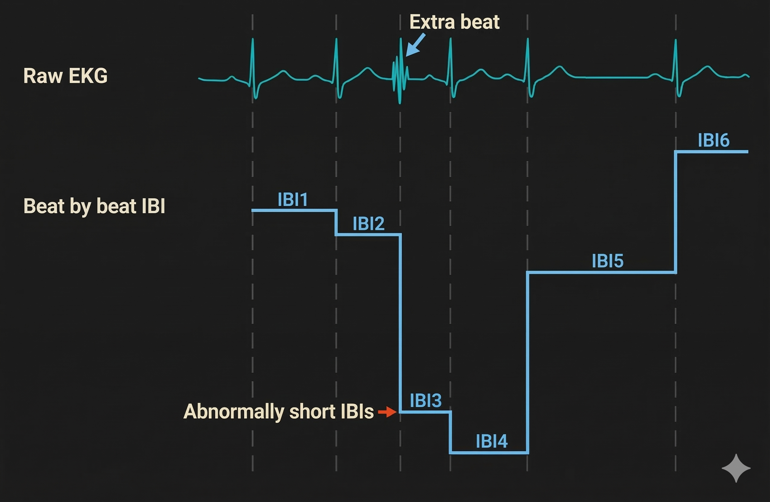
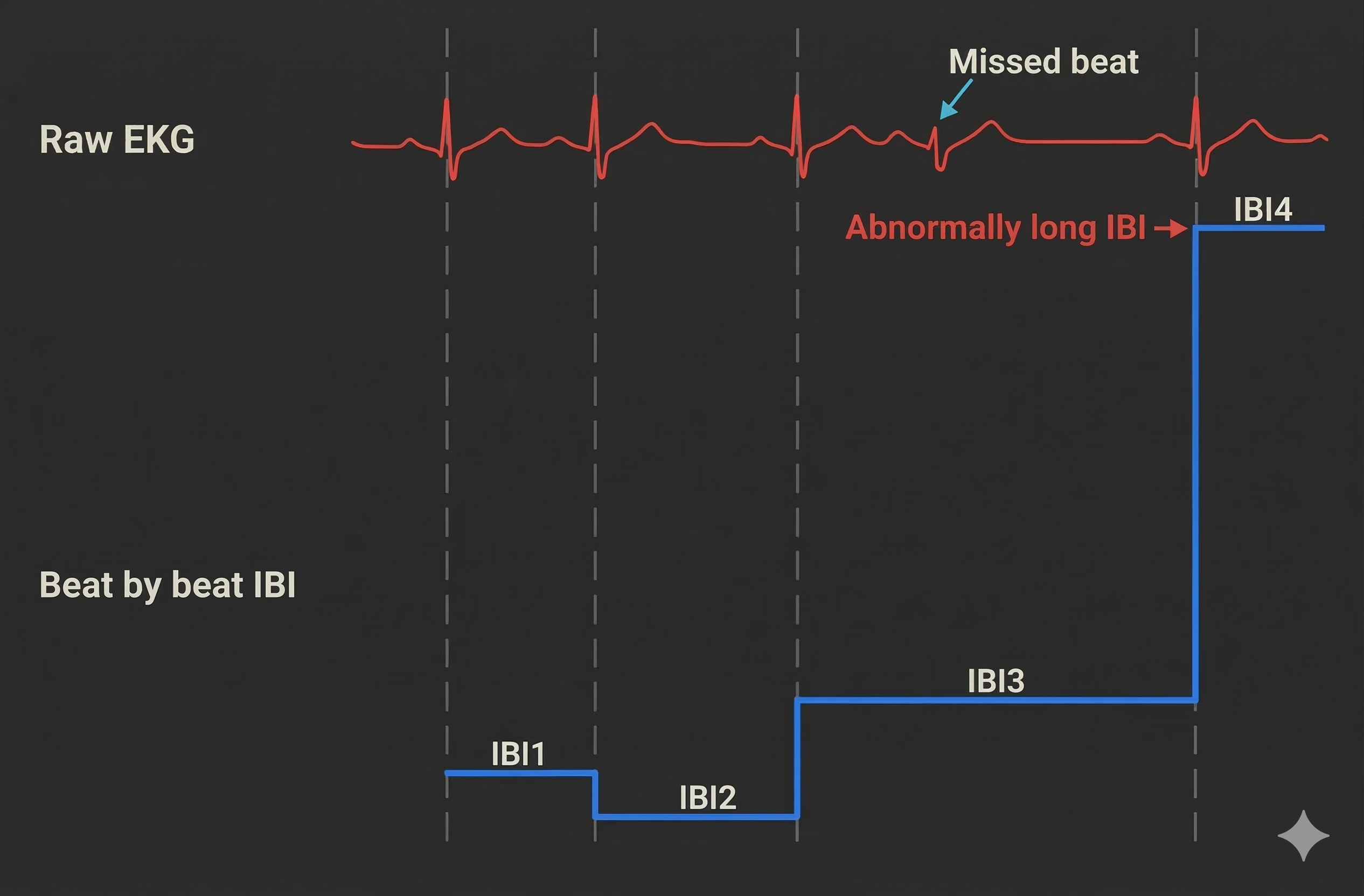
The relationship between artifacts in the raw signal and false IBI values can be challenging for beginners to grasp. For ECG recording, the software analyzes the raw signal to detect R-spikes—the tall, sharp peaks that mark ventricular depolarization—and measures the time intervals between them. When artifacts distort this process, the resulting IBI values no longer reflect true cardiac timing.

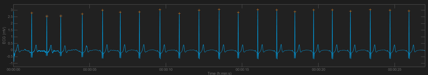
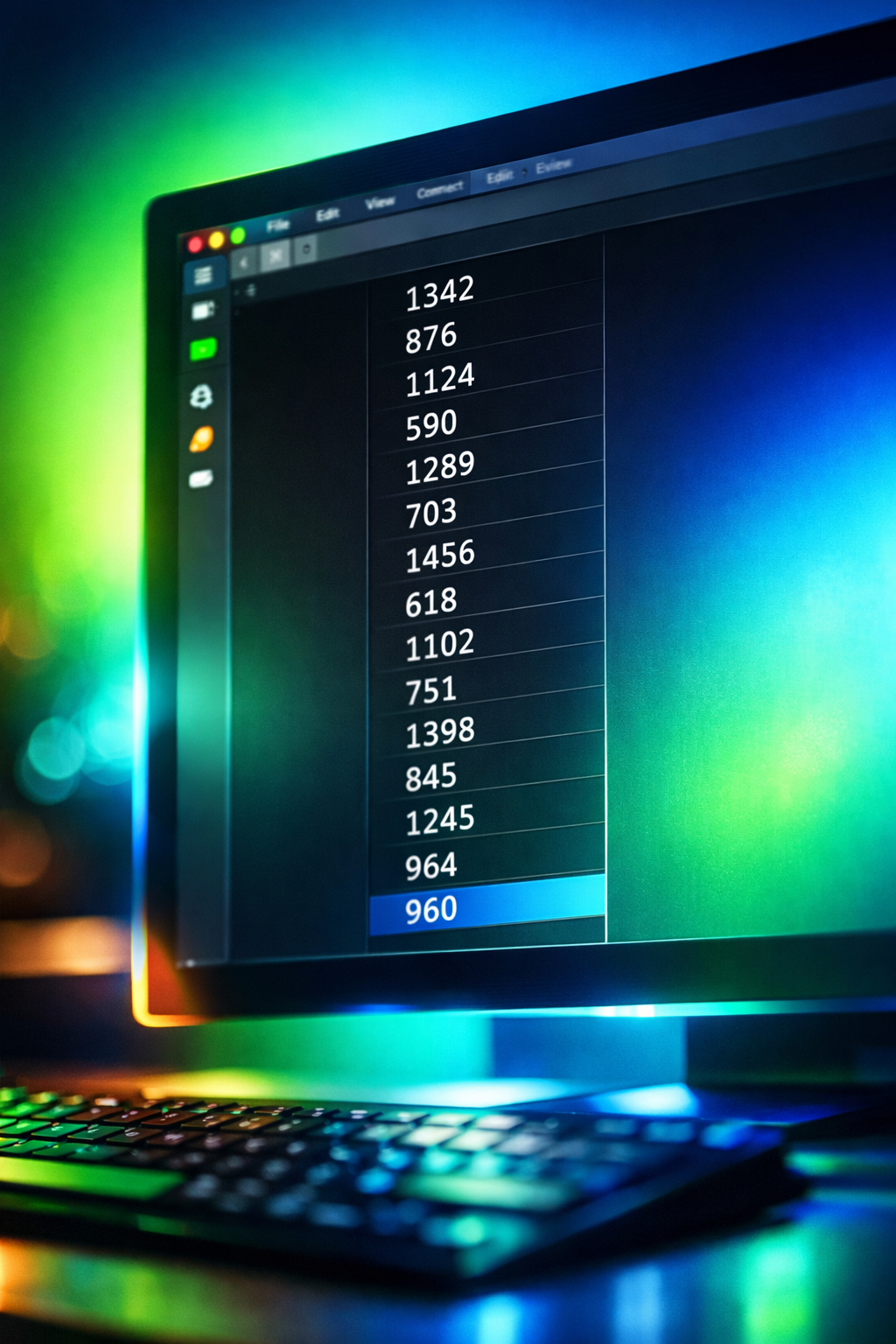
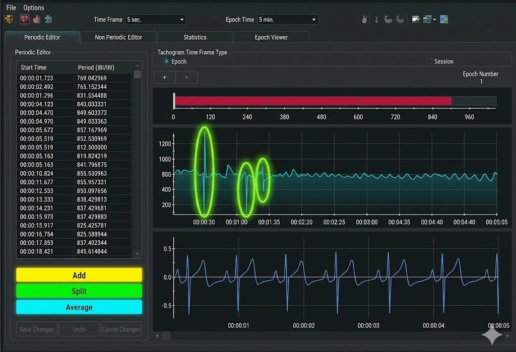
IBIs are stored in a time-stamped table of consecutive values, similar to an Excel spreadsheet column. The ECG waveform circled above at 29.171 milliseconds corresponds to an IBI value of 818.359 milliseconds at the bottom of the table below. Understanding this correspondence is essential for tracing artifacts from their source in the raw signal to their impact on computed metrics.

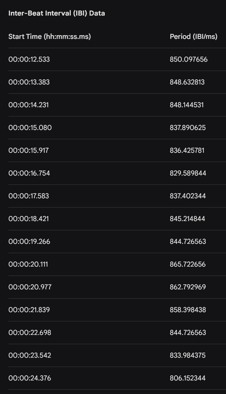
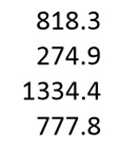
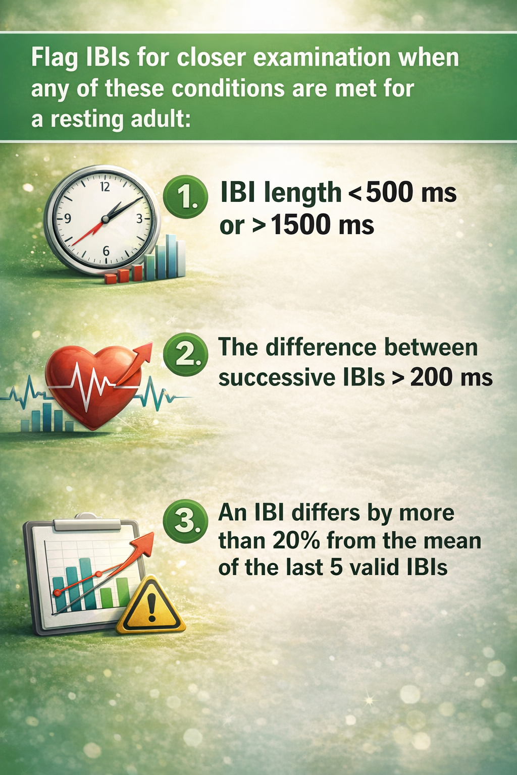
Artifacts can cause the software to "see" extra beats, resulting in abnormally short IBIs. They can also cause it to miss beats, resulting in abnormally long IBIs. These outliers stand out when you review a table of IBI values. For example, we used the color red to identify a short IBI of 274.9 milliseconds produced by an extra beat—far below the typical resting range of 600-1200 milliseconds.

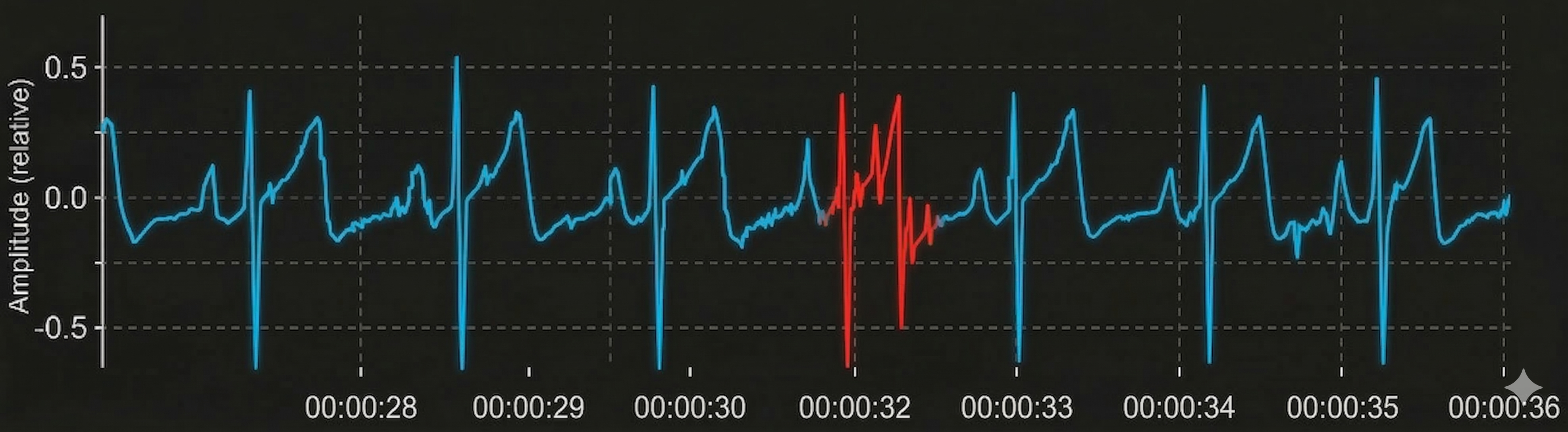
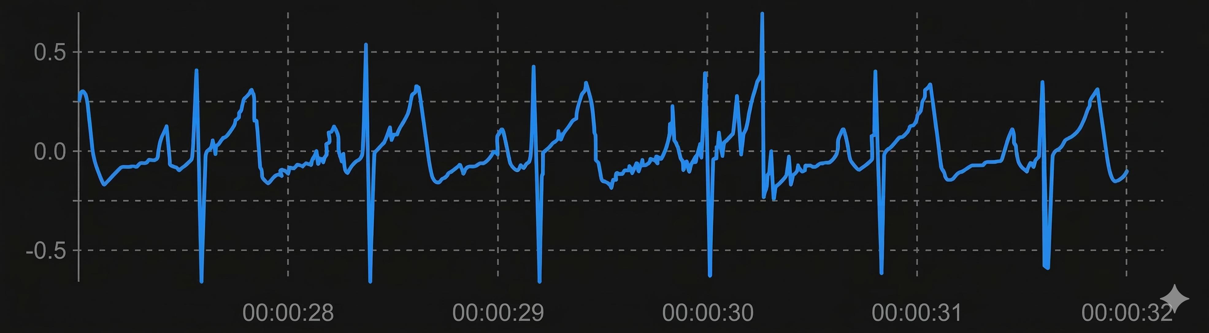
Conversely, software missed a beat before 00:00:31, resulting in a long IBI of 1334.4 milliseconds. When software fails to detect an R-spike, it measures the interval from one detected beat to the next, effectively doubling (or more) the true interval.

Short and long values stand out compared to typical adult values. Developing an eye for these outliers is a fundamental skill for any clinician working with HRV data.

BCIA Blueprint Coverage

This unit addresses III. HRV Instrumentation: E. Artifacting Strategies from the BCIA certification blueprint. Whether you are preparing for certification or expanding your clinical competencies, this material provides the foundation for defensible data quality practices.

Topics include Artifacting Overview, Plan A (Segment Removal and Detrending) and Plan B (Manual Correction and Detrending). Each approach suits different clinical scenarios, and knowing when to apply each one will improve both your efficiency and your data integrity.

🎧 Listen to the Full Chapter Lecture

Artifacting Overview: Understanding the Process

This section introduces the fundamental principles of artifacting and explains why certain correction approaches are inappropriate. You will learn what artifacting is, when data should be discarded, and why the "splicing" method fails to preserve data integrity.

Artifacting is the process of removing or replacing false values found within a data record. Think of it as quality control for your HRV data: you are ensuring that every value in your dataset represents a genuine cardiac event rather than noise or error. This process directly parallels the artifact rejection procedures familiar to clinicians who practice neurofeedback.

Researchers may discard the first and last minutes of data due to client adjustment to the monitoring environment and performance degradation after a long recording session. The initial adjustment period reflects the client settling into the recording situation—electrode gel stabilizing, the client becoming accustomed to the sensors, and initial anxiety subsiding. Toward the end of extended sessions, fatigue and reduced attention can affect data quality, particularly if the client shifts position or loses focus.

The Splicing Method: What Not to Do

Never remove a part of an epoch (a defined data collection period, typically 5 minutes for standard HRV assessment) and rejoin the remaining sections. This approach destroys the temporal relationship between heartbeats, which contains meaningful physiological information (Combatalade, 2010). When you cut out a section and splice the remaining parts together, you create artificial transitions that never occurred in the client's actual cardiac rhythm.

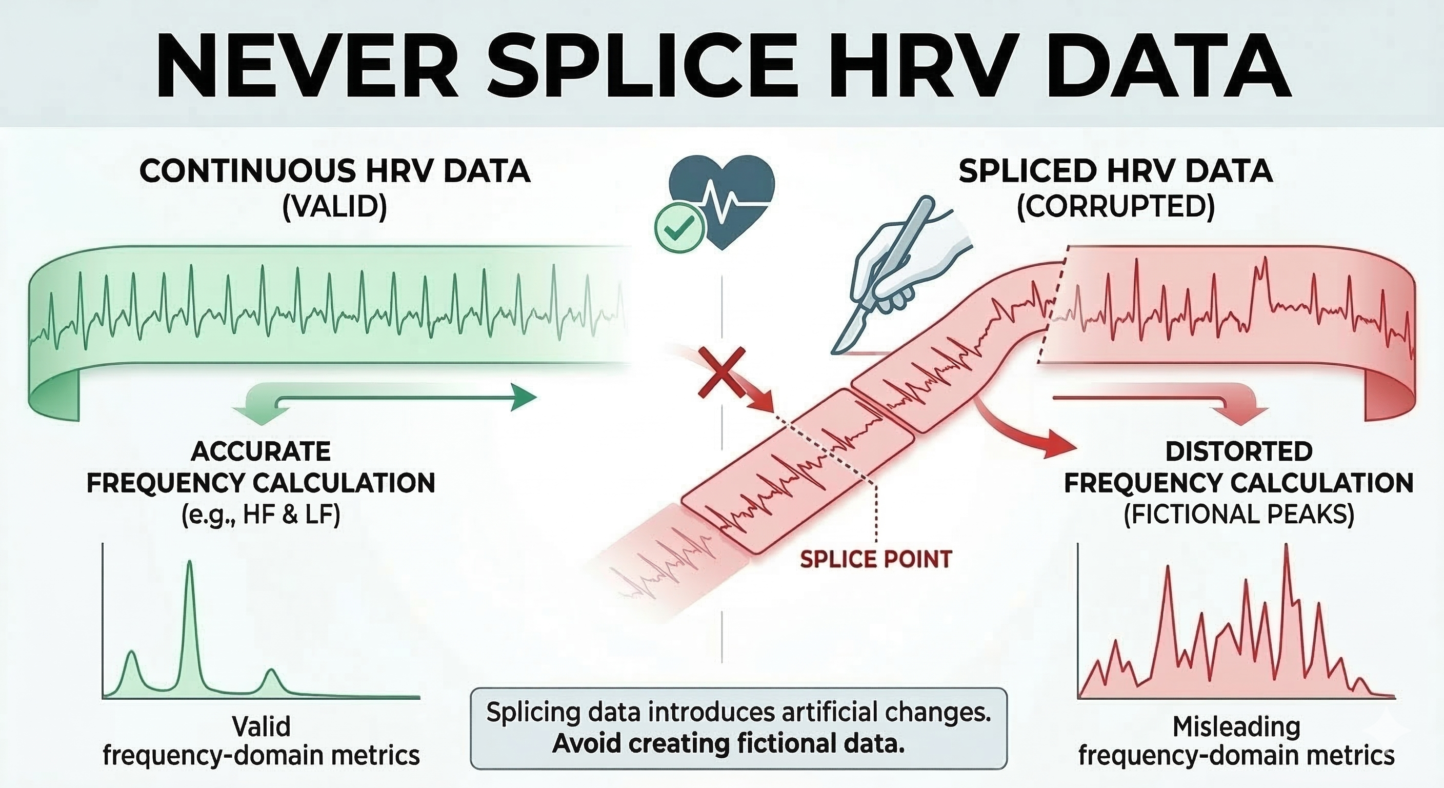
The consequences of splicing are particularly severe for frequency-domain analysis. HRV analysis algorithms expect a continuous time series with natural beat-to-beat relationships. When you splice data together, they interpret the artificial junction as a sudden physiological change, potentially creating spurious power in specific frequency bands that misrepresent your client's autonomic function.

Plan A: Segment Removal and Detrending

This section covers Plan A: when you have sufficient clean data, analyze only the artifact-free segment. You will learn how Kubios Scientific cleans data in two stages (noise detection and beat correction), how deviation thresholds and the automatic correction algorithm work, how cubic spline interpolation repairs identified intervals, and how detrending mathematically restores stationarity using the smoothness priors method.

When an epoch is at least 6 minutes long and the artifact occurs in the first or last 3 minutes, you can analyze the clean 3-minute segment (Gevirtz, 2018). This approach preserves the temporal integrity of your data while avoiding the contaminated portion entirely. The clean segment contains a set of IBI values measured over time—what we call a time series. Visualize this as an Excel column where each cell contains a millisecond value (e.g., 818.3 ms) representing the time between consecutive heartbeats.

Clearing the Static with Noise Detection

Kubios uses a feature called noise detection to act as a high-powered filter for your heart rate data. If a segment of your recording becomes too messy—perhaps because a sensor slipped or you moved suddenly—the software marks that entire block as unreadable. Instead of trying to guess what happened during those distorted moments, it simply sets that section aside so it won't ruin your final results. This tool is essential for handling external interference and ensuring that only the highest quality data makes it through to the final analysis. By removing these large, unreadable chunks, the software protects the accuracy of your heart rate variability scores.

Kubios allows you to select a color-coded clean segment for further analysis, skipping corrupted values.

Polishing the Details with Beat Correction

While noise detection handles the big, messy gaps, beat correction acts like a precision editor for the smaller details. It doesn't throw away whole sections of data but instead looks for tiny, individual hiccups like a single "extra" heartbeat. These brief stutters are often natural or caused by a minor sensor glitch, and the software is smart enough to recognize them. Rather than deleting these moments, beat correction surgically adjusts the timing of those specific intervals to keep the rhythm mathematically consistent. This allows you to keep as much of your heart’s story as possible without one weird beat throwing everything off.

A Two-Step Cleaning Process

These two features work together in a specific sequence to ensure your data is as clean as possible. First, the noise detection clears out the "trash" caused by movement or poor signal quality. Once those big gaps are handled, the beat correction tool goes through the remaining data to smooth out any minor, individual quirks. This two-stage process ensures that the software isn't trying to "fix" something that is actually just pure noise. The result is a polished, reliable picture of your heart's health that reflects your actual physiology rather than technical errors.

Decoding the Noise Level Graph

To see exactly how much work the software did, you can look at the "Noise Level" graph in your final Kubios report. This graph usually appears as a series of bars or a shaded area along the bottom of your heart rate timeline. When the bar spikes or changes color, it indicates a period where the signal quality dropped and the software had to intervene. If you see large sections marked as noise, it might mean your heart rate strap was too loose or your skin was too dry during the recording. Understanding this graph helps you decide if your data is "clean" enough to trust or if you need to try a more stable recording next time.

The Primary Stage of Error Detection

Before any mathematical transformations can occur, the researcher must act as a guardian of the data by identifying and removing outliers. Outliers are any data points that are so far outside the expected range that they are likely mistakes rather than real biological events. In a practical sense, this means scanning the collection of heartbeats for values that are physically impossible.

For a beginner, this involves setting a window of acceptable time between beats—usually between 400 and 1,300 milliseconds. If the software detects a value of 200 milliseconds, these data are likely "noise," which is electrical interference from the environment or the body that the computer mistakenly labeled as a heartbeat. Conversely, a value of 2,000 milliseconds represents data that are likely "missed beats," where the heart actually fired, but the sensor failed to record it. Removing these spikes first is essential because they represent infinite frequency changes that would confuse the software during the next stage.

How Kubios Determines When a Beat Is an Artifact

Kubios HRV Scientific identifies abnormal beats using a statistical method developed by Lipponen and Tarvainen that analyzes the RR-interval time series, which is the sequence of time intervals between successive heartbeats (Lipponen & Tarvainen, 2019). In electrocardiography (ECG), an RR interval is the time between two consecutive R waves, the large spikes that represent ventricular depolarization. In HRV analysis, these intervals form a tachogram, a time series that reflects how heart period fluctuates over time.

The Lipponen–Tarvainen algorithm does not rely on the ECG waveform shape to identify abnormal beats. Instead, it compares each interval to the local rhythm, which is estimated using a short moving window that calculates the expected interval duration based on neighboring beats. If the interval deviates too far from this expected value, Kubios assumes that something abnormal occurred, such as a premature beat, a missed detection, or motion artifact. The degree of deviation that is allowed before a beat is classified as abnormal is called the deviation threshold.

A deviation threshold defines the maximum difference between the observed RR interval and the expected interval that Kubios will accept as normal. When the difference exceeds this threshold, the software labels the beat as an artifact or ectopic event and replaces the abnormal interval using interpolation so that the HRV calculations are based on an estimated sinus rhythm (Lipponen & Tarvainen, 2019).

The Meaning of Deviation Thresholds in Kubios

Kubios provides several artifact-correction strength settings. Each setting corresponds to a specific deviation threshold expressed in milliseconds (ms). One millisecond equals one thousandth of a second. For reference, a typical resting RR interval in a healthy adult is around 600–1200 ms, corresponding to heart rates of about 50–100 beats per minute.

The threshold therefore represents how large a deviation Kubios will tolerate relative to the local rhythm before classifying a beat as abnormal. Larger thresholds allow greater variation and therefore detect fewer artifacts, while smaller thresholds are stricter and detect more artifacts.

No Correction

When the None option is selected, Kubios performs no automatic artifact detection or correction. Every interval detected in the RR series is accepted as valid, regardless of how abnormal it may appear. This setting is rarely appropriate unless the recording has already been manually inspected and edited. Because HRV metrics are highly sensitive to abnormal intervals, even a single premature beat can inflate measures such as RMSSD or SDNN if it is left uncorrected (Shaffer & Ginsberg, 2017).

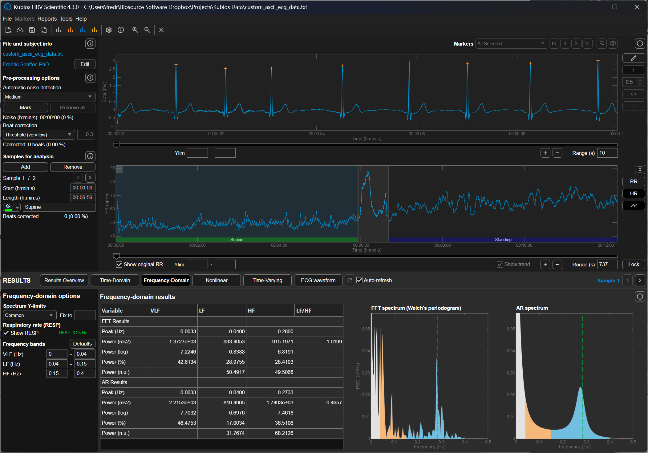
Very Low Correction (±450 ms)

The Very Low correction level allows intervals to deviate by approximately ±450 milliseconds from the expected interval before Kubios flags them as artifacts. In practical terms, this means that an RR interval could be nearly half a second longer or shorter than the surrounding rhythm and still be treated as normal.

This extremely permissive threshold is intended for data sets that contain very large natural variability or when the user wishes to minimize automatic corrections. Because the threshold is so wide, only the most obvious abnormalities, such as missed beats or extremely premature contractions, are detected.

Low Correction (±350 ms)

The Low setting reduces the allowable deviation to approximately ±350 milliseconds. This means that if the expected RR interval is 900 ms, Kubios will flag intervals shorter than roughly 550 ms or longer than about 1250 ms.

At this level, Kubios detects clear ectopic beats or missed detections but still allows relatively large physiological variability. This setting is commonly used for high-quality ECG recordings in which only occasional artifacts are expected.

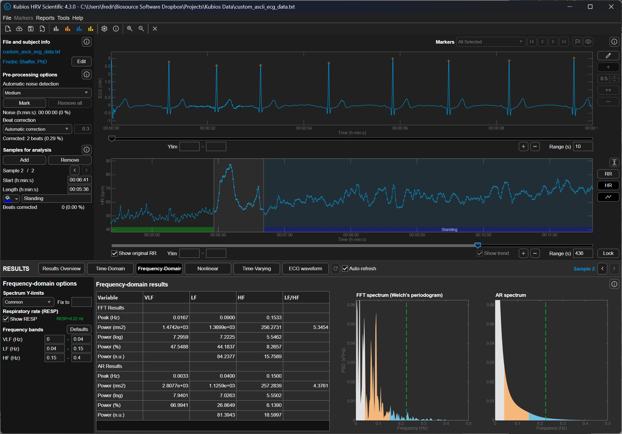
Medium Correction (±250 ms)

The Medium correction level allows a deviation of approximately ±250 milliseconds from the expected interval. In the previous example of a 900 ms rhythm, intervals shorter than about 650 ms or longer than about 1150 ms would be classified as abnormal.

This level represents a balance between sensitivity and conservatism. It detects most premature beats and many motion artifacts while preserving legitimate physiological variability. For many research recordings, particularly those collected under resting conditions, the Medium setting is often recommended.

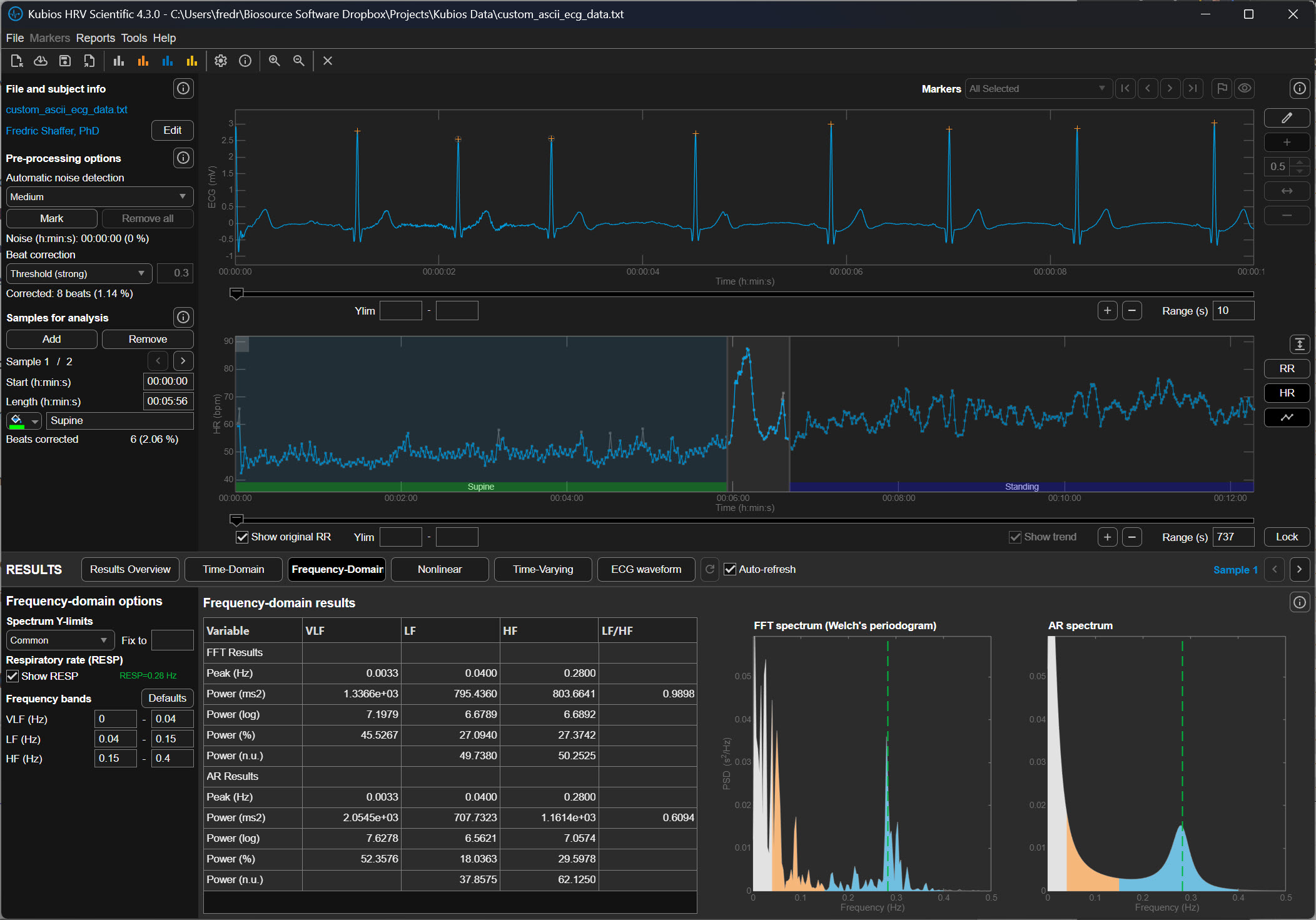
Strong Correction (±150 ms)

The Strong setting tightens the allowable deviation to approximately ±150 milliseconds. If the expected interval is 900 ms, Kubios will flag intervals shorter than about 750 ms or longer than about 1050 ms.

This stricter threshold captures smaller irregularities in the RR sequence and is often used when recordings contain significant noise or motion artifact. However, it can occasionally misclassify legitimate physiological changes as artifacts, particularly during large respiratory sinus arrhythmia, which is the natural fluctuation in heart rate associated with breathing.

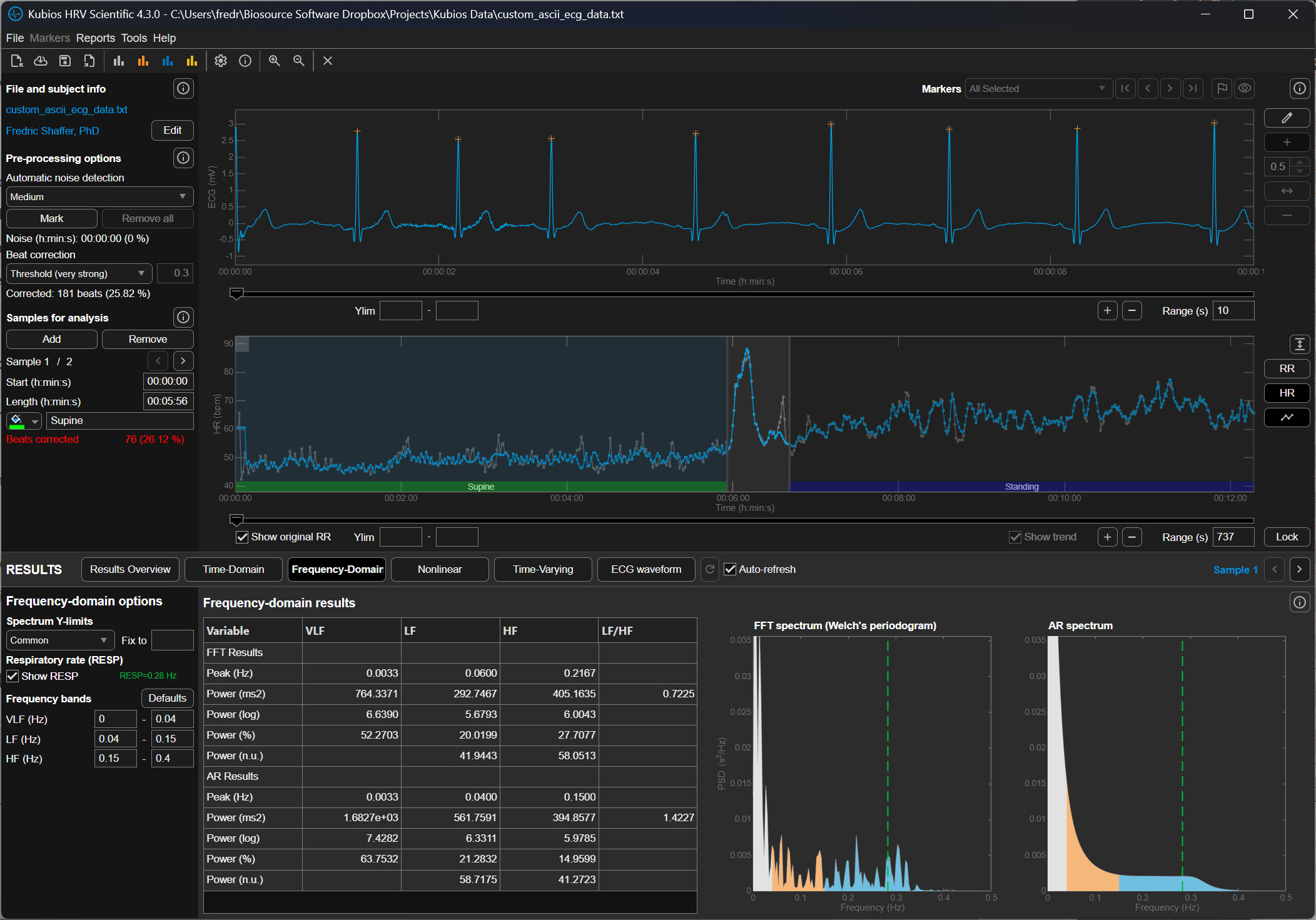
Very Strong Correction (±50 ms)

The Very Strong setting allows only ±50 milliseconds of deviation from the expected interval before Kubios marks a beat as abnormal. In a rhythm of 900 ms, intervals shorter than 850 ms or longer than 950 ms would be corrected.

This extremely strict threshold aggressively removes irregular intervals and is typically used when analyzing noisy signals from wearable photoplethysmography (PPG) devices or recordings contaminated by substantial motion artifact. Because the threshold is so narrow, it can also remove genuine physiological variability if applied to clean data.

Why the Threshold Matters for HRV Analysis

Heart rate variability metrics quantify the natural fluctuations in cardiac timing produced by autonomic regulation of the sinoatrial node. When abnormal beats remain in the data, they artificially increase variability measures such as the RMSSD (root mean square of successive differences) and the SDNN (standard deviation of normal intervals). Conversely, overly aggressive artifact correction can remove legitimate variability and reduce these metrics.

The deviation threshold therefore determines how Kubios balances preserving physiological variability against removing abnormal intervals. Selecting the appropriate setting requires considering the recording quality, the measurement method (ECG versus PPG), and the expected magnitude of heart rate fluctuations.

Practical Perspective

In practical HRV analysis, researchers typically begin with Low or Medium correction for clean ECG recordings. Stronger settings are used when signals contain substantial artifact, particularly in wearable devices where motion interference is common. After correction, analysts should visually inspect the tachogram to ensure that genuine physiological rhythms have not been removed.

Understanding these deviation thresholds helps the user interpret how aggressively Kubios is editing the RR-interval series and how that editing may influence the final HRV metrics.

Automatic Beat Correction

The automatic system provides a standardized, repeatable way to ensure that every file in a study is treated exactly the same way, which is vital for the scientific validity of research.

How Kubios' Automatic Algorithm Thinks

The reason Kubios developers favor the automatic method over older, manual thresholds is its ability to adapt to the unique rhythm of the individual. Traditional methods often use a fixed threshold, such as a rule that flags any beat that is 20% different from its neighbor. However, a fixed rule like this can be problematic; it might be too strict for an athlete with a very dynamic heart or too loose for an elderly patient with a very steady rhythm. The automatic algorithm instead uses a time-varying approach, which means it constantly recalculates what a "normal" change looks like based on the heartbeats immediately surrounding the current one. It essentially learns the "language" of that specific heart in real-time, allowing it to distinguish between a natural, healthy jump in heart rate and a technical glitch.

Precision in Identifying Ectopic Beats

One of the most difficult challenges for a beginner is identifying ectopic beats, which are premature heartbeats that originate from a different part of the heart than the standard pacemaker. While these are real physical events, they act as statistical outliers that can ruin heart rate variability calculations. Kubios recommends the automatic setting because it is incredibly precise at identifying these specific patterns. Kubios does not examine waveform morphology (i.e., shape). Instead it examines interval lengths. The software looks for a very short interval followed immediately by a long, "compensatory" pause— a classic signature of an ectopic beat. By automatically detecting these, the software can remove the influence of the irregular beat while accurately estimating what the heart's rhythm would have been if the interruption hadn't occurred.

The Role of Cubic Spline Interpolation

Once the automatic system identifies an error, it doesn't just leave a hole in the data. Kubios uses a sophisticated technique called cubic spline interpolation to heal the gap. To understand this, imagine you have a series of dots on a page representing heartbeats, and one dot is missing. Interpolation is the process of drawing a smooth, curved line between the existing dots to estimate where the missing dot should have been. A cubic spline is just a specific mathematical way of drawing that curve so that it remains perfectly smooth and follows the natural acceleration and deceleration of the heart. Kubios recommends the automatic system because it performs this complex math instantly and accurately, ensuring that the final data set remains continuous and ready for analysis.

Practical Reliability for Modern Research

Ultimately, the recommendation for automatic correction comes down to its proven reliability across thousands of different types of recordings. In formal testing, this algorithm has shown nearly 100% accuracy in finding missed or extra beats, which are the most common errors in heart rate data.

For a beginner, this provides a safety net that allows you to focus on interpreting your results rather than worrying about whether you manually clicked the right button on a jagged graph. By trusting the automatic process, you are using a tool that has been refined through years of peer-reviewed research, ensuring that your data are as clean and accurate as possible before you draw any conclusions about the body's physiological state.

Although applications like Kubios have become increasingly refined, beginners and experienced professionals should always "trust, but verify" by examining the the resulting tachogram (beat-to-beat map) for artifacts.

Understanding Trends in HRV Data

Once the sharpest errors have been scrubbed away, the data are ready for the second stage: detrending. To understand detrending, one must first understand stationarity. In heart rate research, we prefer that our data be stationary, meaning their average value and their variance stay relatively constant over time.

During long measurement periods, there is often a gradual change in the mean or variance of IBI values, called a trend. Trends occur for various physiological and environmental reasons.

Human bodies are naturally non-stationary. If a person breathes deeply or shifts their weight, the heart rate may slowly drift upward or downward over several minutes. This slow drift is called a trend. If we left these trends in the data, they would appear as massive waves in our final analysis, drowning out the faster, more subtle heart rate changes we actually want to measure. Detrending is the technical process of identifying this slow, underlying drift and subtracting it from the data so that the remaining heartbeats sit on a level, horizontal line.

Trends can violate the stationarity assumption underlying many HRV analysis methods. Stationarity means that the statistical properties of the IBI values—such as the mean and standard deviation—do not change systematically over time. When this assumption is violated, frequency-domain metrics may not accurately reflect underlying autonomic function because the algorithm cannot distinguish between true oscillatory patterns and the drift superimposed upon them.

The graphics below illustrate acceptable versus weak stationarity (adapted from Kubios). In the acceptable case, statistical properties remain relatively stable throughout the recording. In the weak stationarity example, some drift is present but may still be acceptable depending on your clinical purposes and the specific metrics you need.

Detrending: Removing Systematic Changes

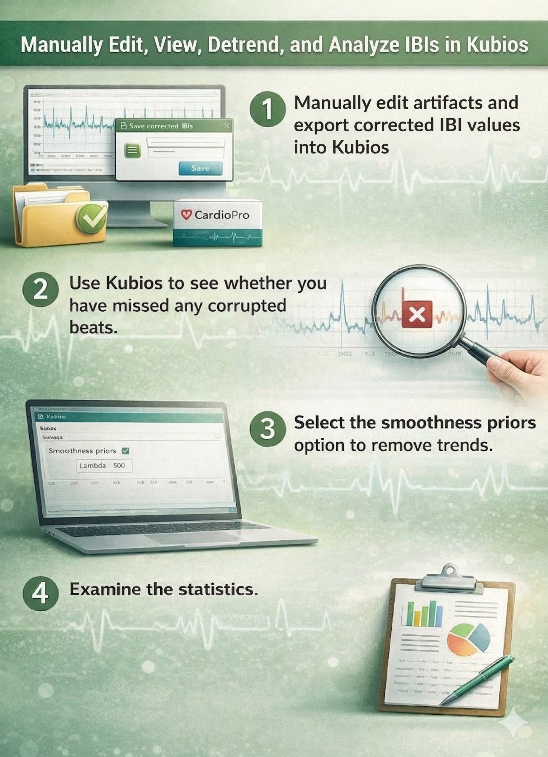
Detrending is the mathematical removal of a trend from a time series to ensure stationarity. Kubios provides a smoothness priors function for this purpose, allowing you to select the smoothness of the removed trend by entering a lambda value. Lambda is the smoothing factor; higher values remove smoother (lower-frequency) trends. Kubios displays the corresponding cutoff frequency beside the lambda value you enter, helping you understand exactly what you are removing.

Implementing Smoothness Priors in Practice

In Kubios, smoothness priors is a sophisticated digital filter that acts like a flexible ruler held against the data points. The software calculates a smooth, curving line that follows the general trend of the heart rate without being distracted by the quick, beat-to-beat changes.

This smooth line represents the noise of the body’s slow drifts. Once this line is calculated, the software performs a subtraction: it takes the original data and removes the values represented by that smooth line. What remains are detrended data where every heartbeat is measured against a stable baseline. This ensures that when we later look at the frequencies of the heart—such as those associated with breathing or stress—we are looking at the pure rhythm of the heart's internal clock rather than the slow physical movements of the person being tested.

Adjusting Filter Intensity

When setting up this process, a beginner will encounter a technical parameter known as lambda. Lambda is the setting that determines how stiff or flexible that digital ruler should be. If the lambda is set very high, the ruler is stiff and only removes the very slowest, most gradual drifts.

If the lambda is set low, the ruler becomes more flexible and starts to follow even the quicker changes in heart rate. For most standard research, a lambda of 500 is the gold standard because it is specifically tuned to ignore any movement that happens slower than about 0.035 Hertz, which is a technical way of saying it ignores anything that takes longer than 30 seconds to complete one cycle. By keeping this setting consistent, researchers ensure that they are only removing the non-biological drift while preserving the rapid fluctuations that reveal how the nervous system is responding to the world.

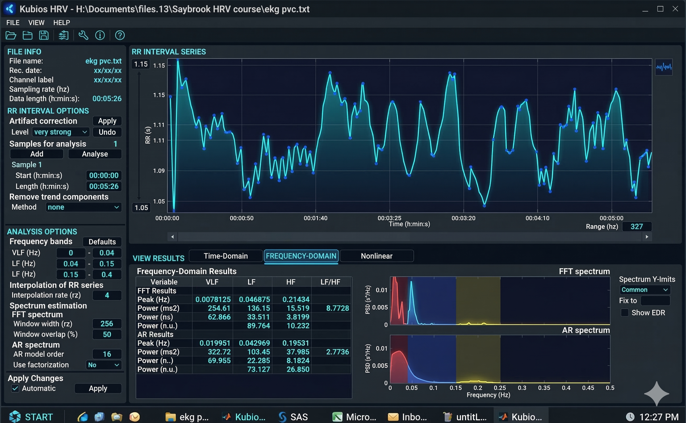
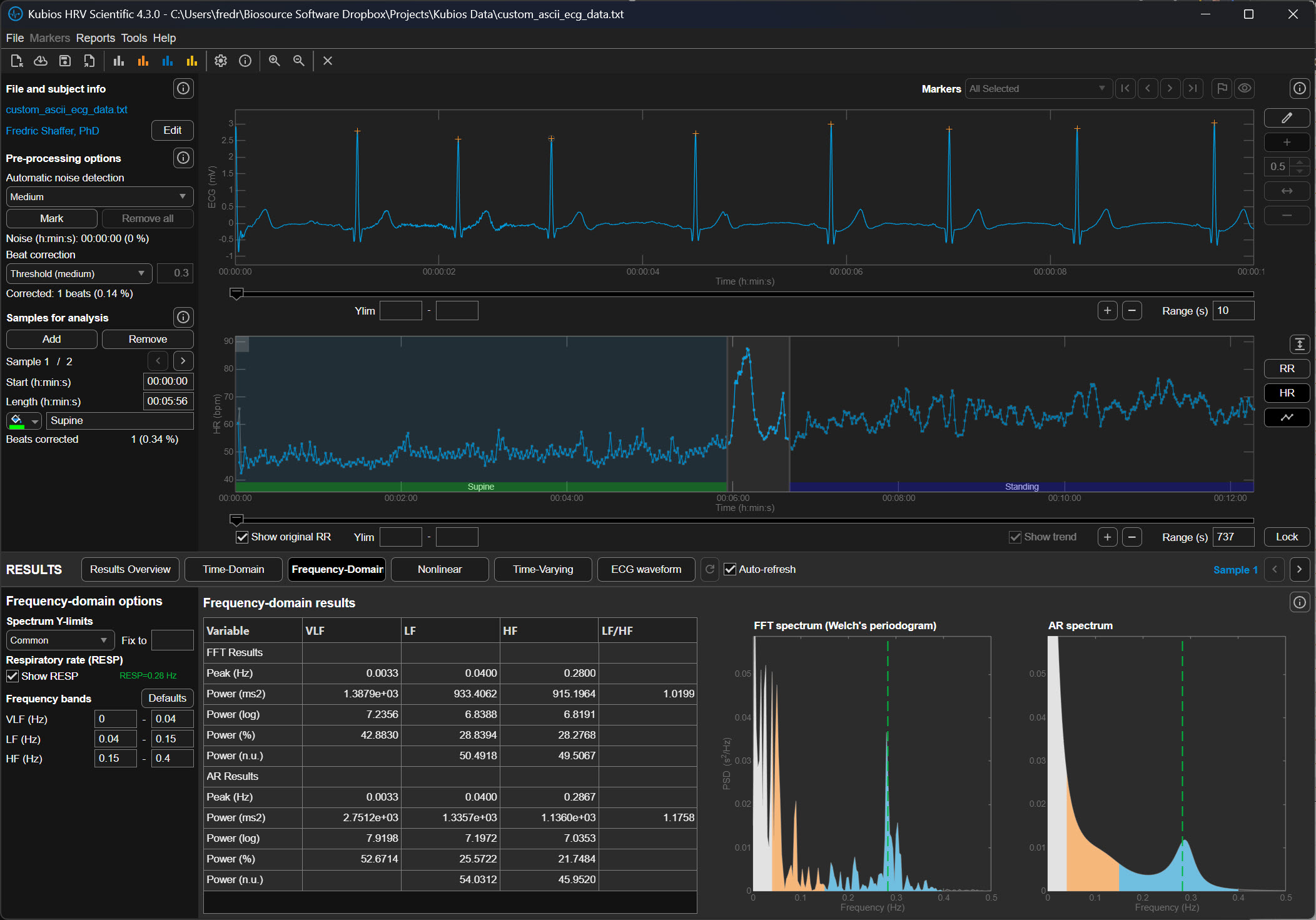
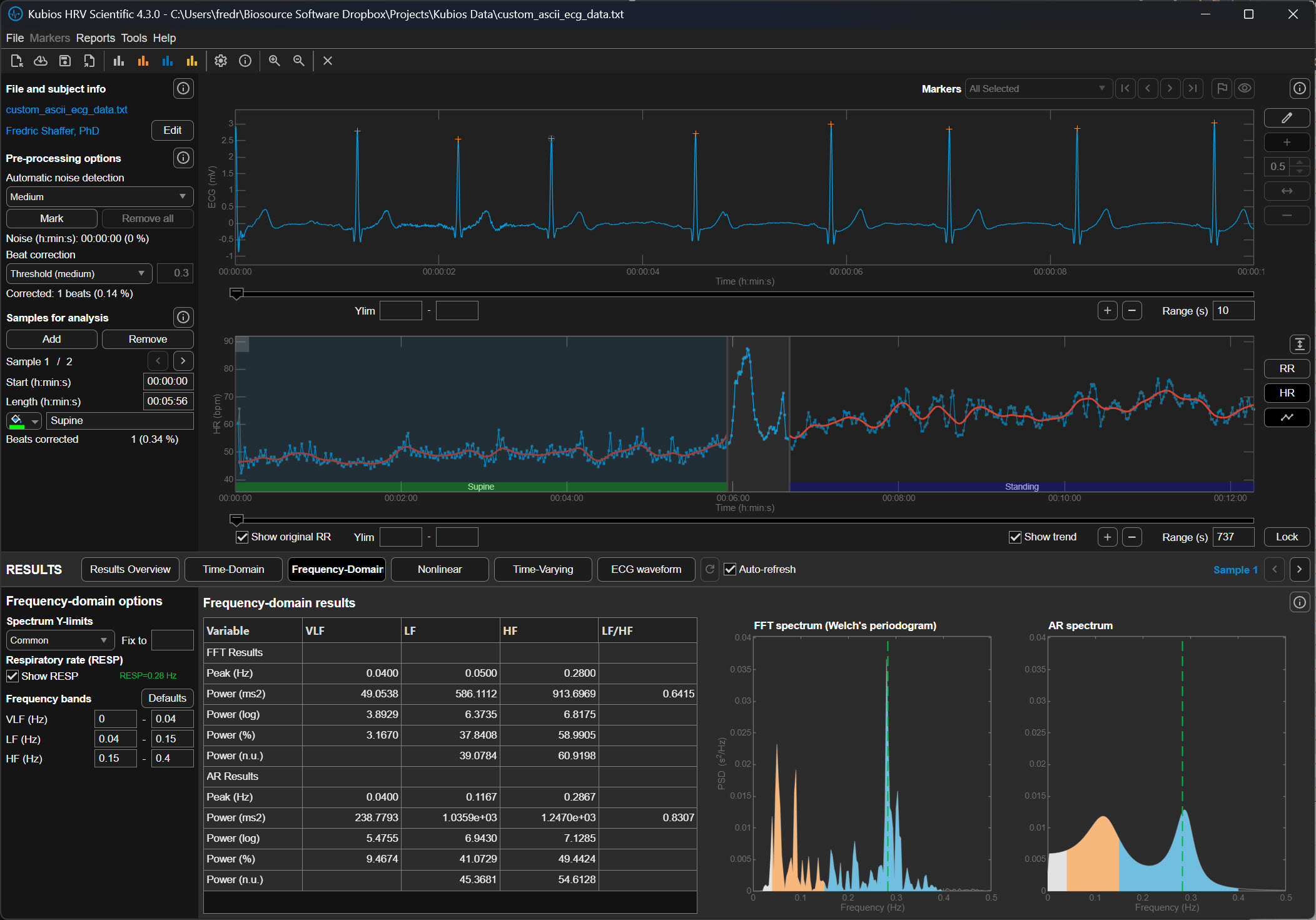
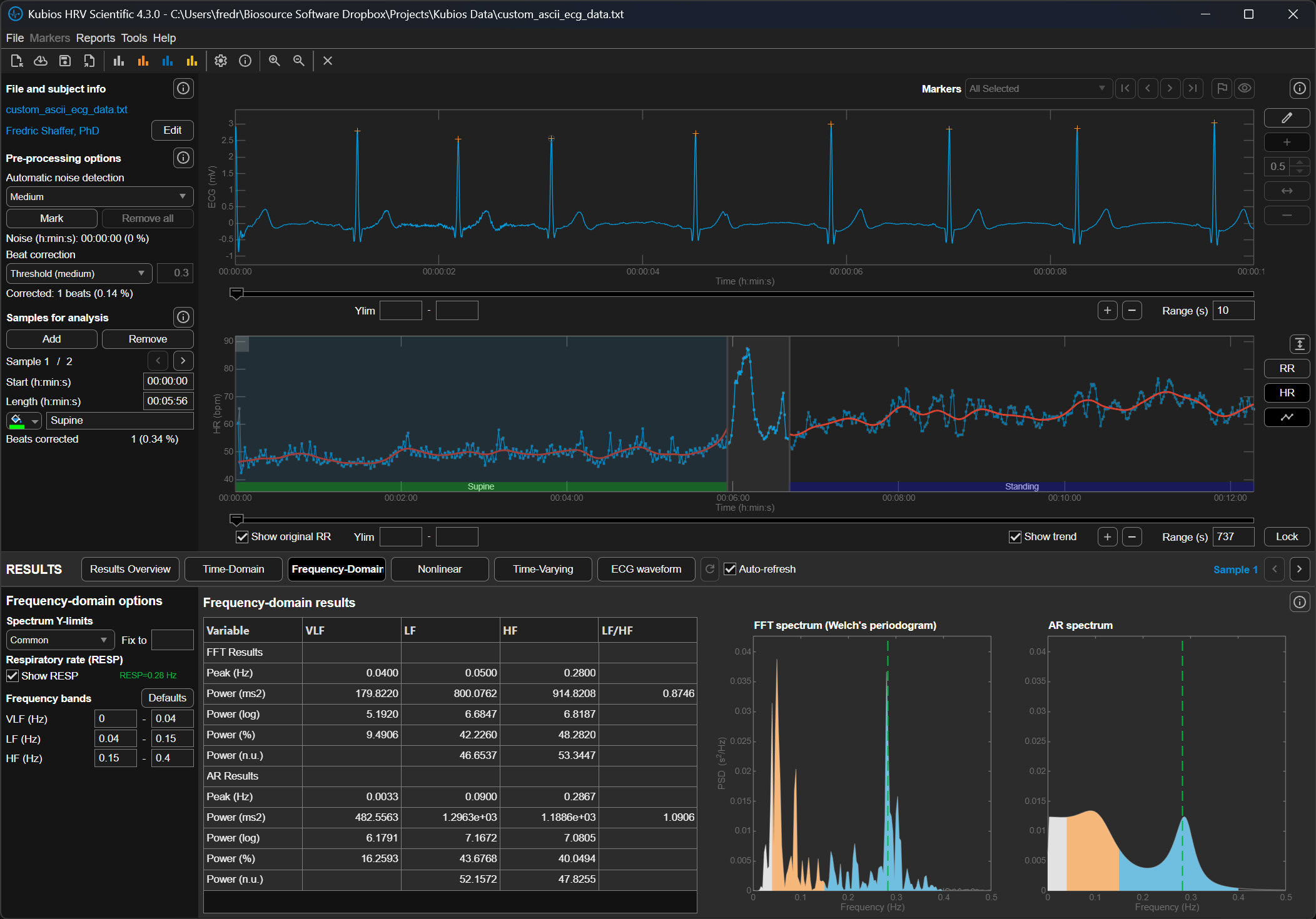
The following graphics demonstrate how different lambda values affect the FFT spectrum (Tarvainen & Niskanen, 2020). All lambda values markedly reduce VLF power (0-0.04 Hz) and may also lower LF power (0.04-0.15 Hz). Understanding this trade-off is essential: aggressive detrending can inadvertently remove genuine physiological variation along with the unwanted trend.

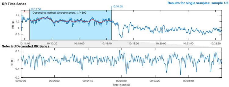
The upper section of the detrending graphic below shows the original time series with a smoothed trend (red line). The lower section shows the same RR series with the trend removed. Notice how the mean becomes stable after detrending—you can draw a straight horizontal line through the mean values, indicating that the systematic drift has been eliminated while preserving the beat-to-beat variability you need to analyze.

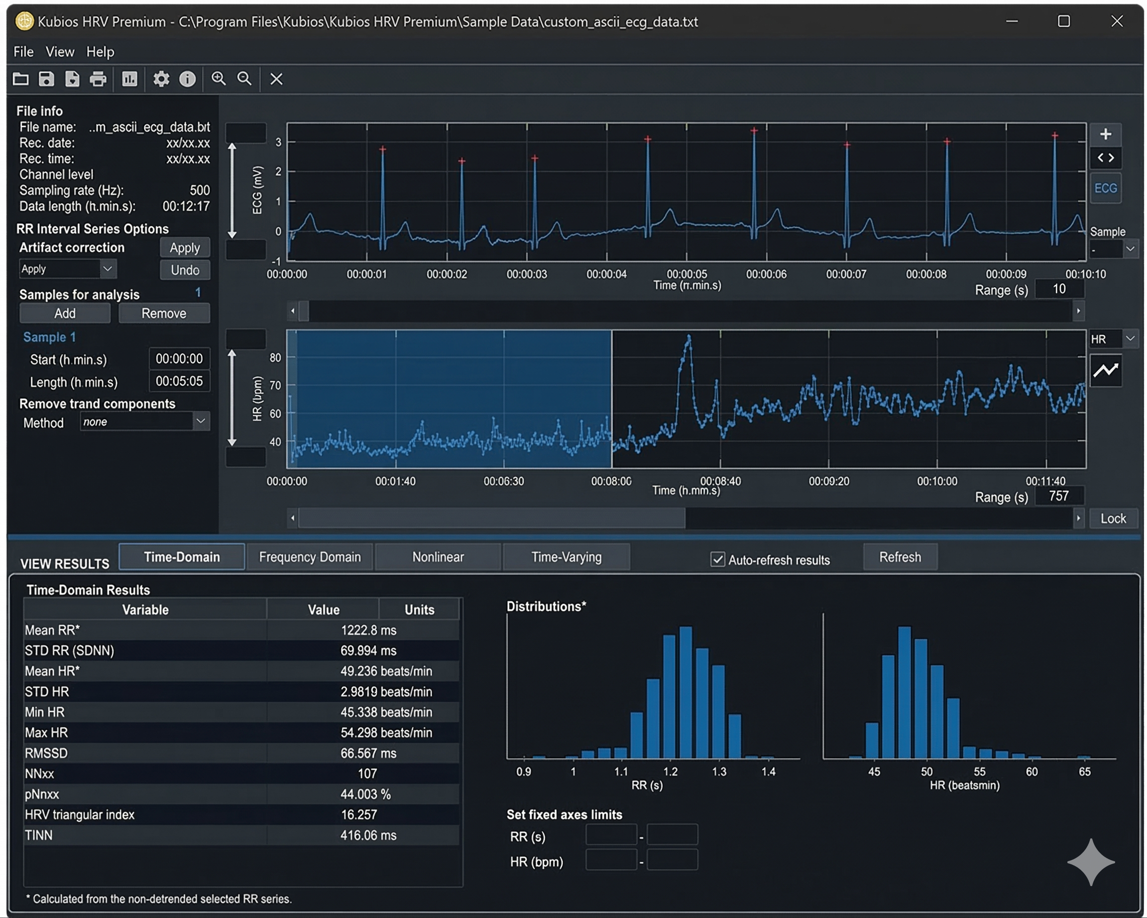
Executing the Workflow in Kubios Scientific

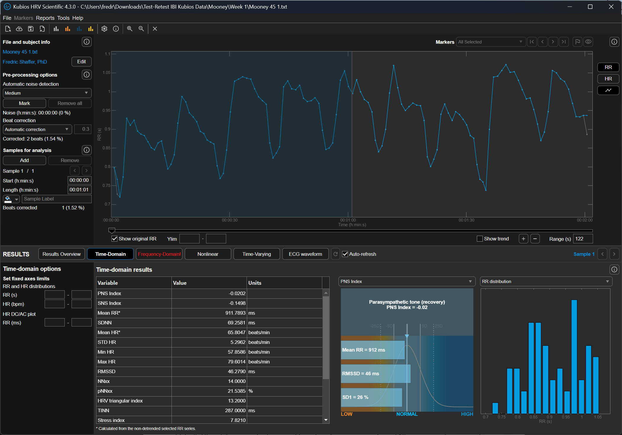
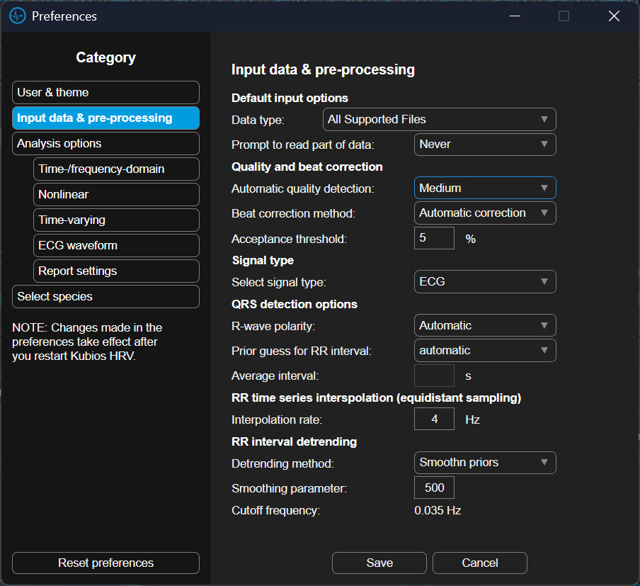
To begin this process in the Kubios Scientific interface, you first open your data file and look to the left-hand side of the screen where the analysis settings are housed. You will first click on the Artifact Correction section to address your outliers. In the dropdown menu, you can select a correction level, such as "Strong" or "Very Strong," which uses the software’s algorithms to compare each beat to its neighbors and automatically replace the outliers with estimated values.

Once these data are corrected, you move your mouse to the "Trend Removal" or "Detrending" section immediately below. Here, you will click the dropdown menu and select "Smoothness Priors." After making this selection, you will see a small box labeled "Lambda." You should ensure this value is set to 500 for a standard five-minute recording. Once these selections are made, the software will process the data, first purging the outliers and then smoothing the trends, leaving you with a clean, level signal ready for final interpretation.

A Practical Perspective

This section addresses the reality that clinical practice often differs from research protocols. You will learn how to balance thoroughness with efficiency, when simplified approaches are appropriate, and how to develop practical artifacting skills through mentorship.

Artifacting is as vital in HRV biofeedback as it is in neurofeedback. However, the intensive data analysis required for publication-quality research may exceed what routine clinical practice demands. The key distinction lies in your purpose: research requires demonstrable data integrity to withstand peer review, while clinical practice requires data quality sufficient to support valid treatment decisions. Both matter, but they involve different standards and workflows.

Clinicians can often limit their review to pre- and post-baseline recordings rather than scrutinizing every training session. You may not need to detrend 5-minute datasets if you can find 3 consecutive minutes of clean data—the Task Force of the European Society of Cardiology (1996) established this as the minimum for valid short-term HRV assessment. If artifacts have corrupted all 5 minutes, examine automatic artifacting within your analysis software and reserve manual artifacting for cases where automated methods prove inadequate.

Artifacting skills can be readily mastered through guidance from an experienced mentor. Contact the Biofeedback Certification International Alliance (BCIA) or your equipment vendor for mentor recommendations. A skilled mentor can help you develop clinical judgment about when to invest additional time in careful artifacting versus when simpler approaches suffice.

Plan B: Manual Correction and Detrending

This section covers manual artifact correction, the gold standard when automated methods are insufficient. You will learn to use visualization tools for artifact identification, understand the physiology of ectopic beats, and master specific correction strategies for different artifact types.

Manual correction and detrending is the best approach when you cannot find a clean 5-minute or longer segment and fewer than 5% of all beats are corrupted (Berntson & Stowell, 1998). Pre-process your data using Excel or a dedicated HRV analysis program like Thought Technology's CardioPro®. This threshold exists because beyond 5% corruption, even careful manual correction may not produce data that accurately represents the client's true autonomic function.

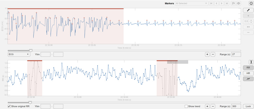
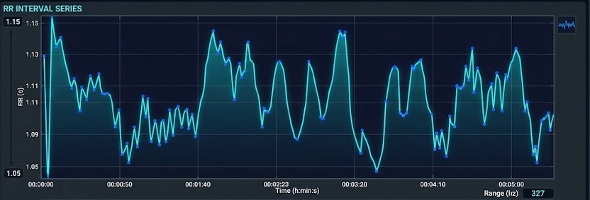
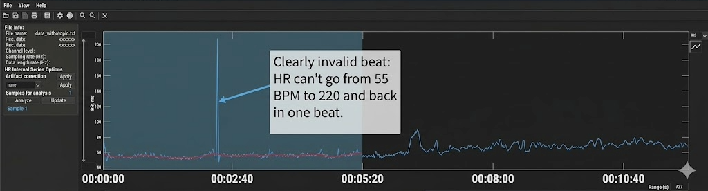
Kubios' Time-Domain tab heart rate plot helps you visualize invalid beats (Gevirtz, 2018). The plot displays heart rate over time, and artifacts typically appear as dramatic spikes or drops that deviate sharply from surrounding values. Because heart rate is the inverse of IBI (HR = 60,000/IBI in ms), a missed beat appears as a sudden heart rate drop, while an extra beat appears as a sudden spike.

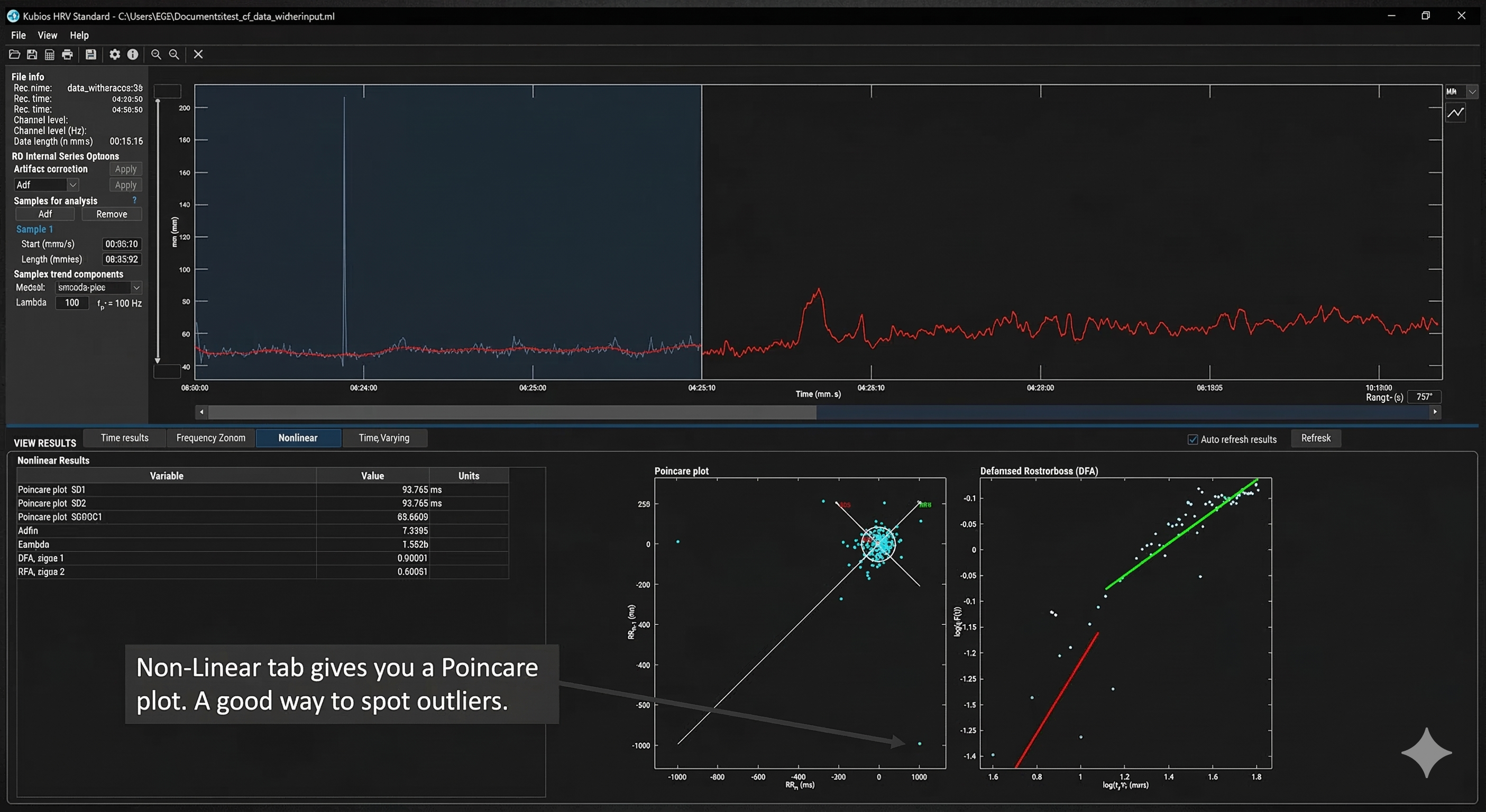
Kubios' Non-Linear tab provides a Poincaré plot, a powerful tool for identifying false beats (Gevirtz, 2018). In a Poincaré plot, each IBI is plotted against the subsequent IBI, creating a visual map of beat-to-beat variability. Normal beats cluster together in an elliptical pattern oriented along a 45-degree line of identity. Artifacts appear as outliers—points that fall far from this main cluster, making them immediately visible even when they might be difficult to spot in a simple time-series display.

Correcting Extra Beats and Missed Beats

Understanding the two fundamental artifact patterns is essential for appropriate correction. Adjacent skeletal muscle activity (SEMG) or ectopic beats produce extra beats that appear as very short IBIs. When the software incorrectly detects a non-cardiac event as a heartbeat, it generates two artificially short intervals where one normal interval should exist. Think of it as the software "seeing" a beat that isn't really there, splitting one true interval into two false ones.

Conversely, when the pulse wave (BVP) peak or R-spike (ECG) amplitude is too low for software recognition, the result is missed beats that appear as prolonged IBIs. The software fails to detect a genuine heartbeat, measuring from one detected beat to the next, effectively skipping the missed one. This commonly occurs with low-amplitude R-spikes, poor electrode contact, or excessive movement.

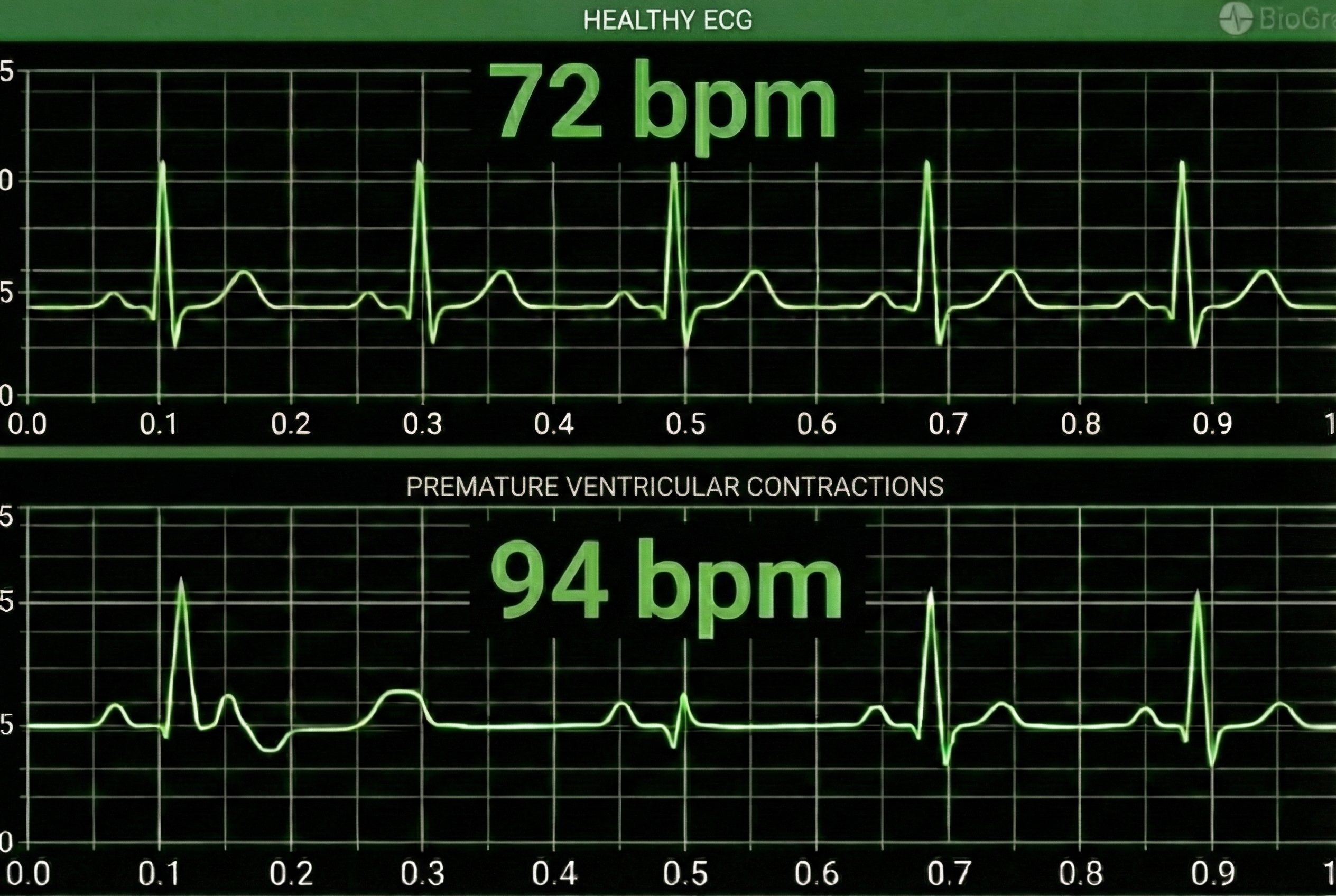
Premature Ventricular Contractions and Their Consequences

Premature ventricular contractions (PVCs) originate from an ectopic focus in the ventricles rather than the sinoatrial node. The heart's normal rhythm is briefly disrupted: an early ventricular depolarization produces a short interval, followed by a compensatory pause while the cardiac electrical system resets to its normal rhythm. This produces a characteristic short-long pattern that is recognizable once you know what to look for.

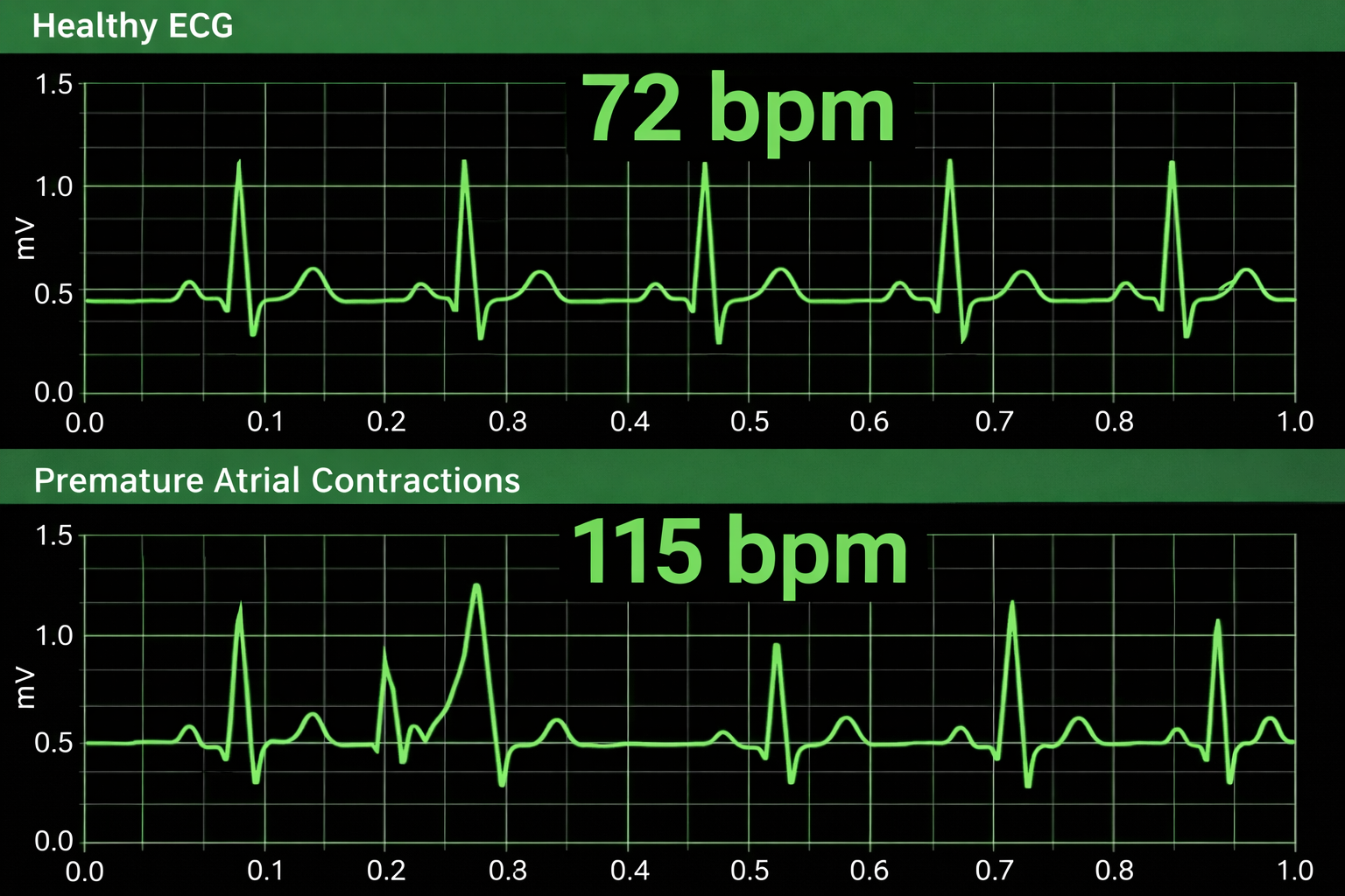
Premature atrial complexes (PACs) are initiated by an ectopic pacemaker in the atria rather than the ventricles. Since PACs involve an extra beat without a compensatory pause, there is no easy way to remove them through manual artifacting (Clinical EEG Interpretation, 2018). PACs are more challenging to correct because they don't produce the symmetrical long-short pattern that makes PVCs relatively straightforward to address.

Manual Correction Strategies

Effective manual correction requires matching the correction strategy to the artifact type. The three primary operations—Add, Split, and Average—each address different patterns of data corruption.

In CardioPro's data editing window (shown below), the Add, Split, and Average options appear at the bottom left. Highlight the abnormal beats (circled in blue) and select the appropriate correction. The Add function combines two consecutive short IBIs into one normal IBI—use this for extra beats. The Split function divides one long IBI into two normal IBIs—use this for missed beats. The Average function replaces abnormal values with an average of surrounding normal values—use this for PVCs and other patterns where the total time should remain constant.

At the current state of the art, expert manual editing can be superior to automated editing. While automated algorithms continue to improve, experienced clinicians can make nuanced judgments about artifact correction that software cannot replicate. Manual editing allows you to consider context—was the client moving, coughing, or talking during that segment? Is this pattern consistent with PVCs versus a missed beat? These contextual factors inform optimal correction choices.

Assignment

Now that you have completed this module, review the missed beat and extra beat graphics and see whether you can identify abnormally long and short IBIs. Based on this module, how might you improve your artifacting practice? Consider the following questions as you reflect on your learning.

First, think about your current recording setup. What steps could you take to prevent artifacts before they occur? Consider factors like sensor placement, environmental interference from nearby electronics, and client preparation including skin cleaning and minimizing movement.

Second, evaluate your current artifacting workflow. Are you using the most appropriate plan (A or B) for your typical recording scenarios? What conditions would prompt you to switch between plans?

Third, consider how you would explain the importance of data quality to a client who is impatient with the careful setup procedures required for clean recordings. How can you help them understand that taking an extra minute for proper preparation ultimately produces more valid and useful results?

Acknowledgment

This article draws heavily on graphics published in Didier Combatalade's Basics of Heart Rate Variability Applied to Psychophysiology (Thought Technology Ltd.) and Tarvainen and Niskanen's Kubios HRV User's Guide. A special thanks to Dr. Richard Gevirtz for sharing Alliant University's artifacting protocol. Dr. Gevirtz is a gifted clinician, educator, and researcher whose contributions have shaped our understanding of HRV biofeedback.

Glossary

References

Altini, M. (2016). Issues in heart rate variability (HRV) analysis: Motion artifacts & ectopic beats. HRV4Training Blog. https://www.hrv4training.com/blog/issues-in-heart-rate-variability-hrv-analysis-motion-artifacts-ectopic-beats

Berntson, G. G., Bigger, J. T., Jr., Eckberg, D. L., Grossman, P., Kaufmann, P. G., Malik, M., Nagaraja, H. N., Porges, S. W., Saul, J. P., Stone, P. H., & Van Der Molen, M. W. (1997). Heart rate variability: Origins, methods, and interpretive caveats. Psychophysiology, 34, 623-648.

Berntson, G. G., & Stowell, J. R. (1998). ECG artifacts and heart period variability: Don't miss a beat! Psychophysiology, 35, 127-132. PMID: 9499713

Cherif, S., Pastor, D., Nguyen, Q.-T., & L'Her, E. (2016). Detection of artifacts on photoplethysmography signals using random distortion testing. 38th Annual International Conference of the IEEE Engineering in Medicine and Biology Society (EMBC). https://doi.org/10.1109/EMBC.2016.7592148

Clinical EEG Interpretation. (2018). Premature ventricular contractions (premature ventricular complex, premature ventricular beats). https://ecgwaves.com/premature-ventricular-contractions-complex-beats-ecg/

Combatalade, D. (2010). Basics of heart rate variability applied to psychophysiology. Thought Technology Ltd.

Combatalade, D. (2013). CardioPro Infiniti: HRV analysis module for BioGraph Infiniti. Thought Technology Ltd.

Elgendi, M. (2012). On the analysis of fingertip photoplethysmogram signals. Current Cardiology Reviews, 8, 14-25. https://doi.org/10.2174/157340312801215782

Gevirtz, R. (2018). Personal communication about artifacting.

Kuusela, K. (2013). Methodological aspects of heart rate variability analysis. In M. V. Kamath, M. A. Watanabe, & A. R. M. Upton (Eds.), Heart rate variability (HRV) signal analysis. CRC Press.

Langner, P. H., Jr., & Geselowitz, D. B. (1960). Characteristics of the frequency spectrum in the normal electrocardiogram and in subjects following myocardial infarction. Circulation Research, 8, 577-584.

Lehrer, P. (2018a). Heart rate, interbeat interval, and the electrocardiogram (shared presentation).

Lehrer, P. (2018b). Personal communication about artifacting.

Lin, I.-M., & Peper, E. (2009). Keep cell phones and PDAs away from EMG sensors and the human body to prevent electromagnetic interference artifacts and cancer. Biofeedback, 37(3), 114-116. https://doi.org/10.5298/1081-5937-37.3.114

Nederend, I., Jongbloed, M. R. M., de Geus, E. J. C., Blom, N. A., & ten Harkel, A. D. J. (2016). Postnatal cardiac autonomic nervous control in pediatric congenital heart disease. Journal of Cardiovascular Development and Disease, 3(2), 16. https://doi.org/10.3390/jcdd3020016

Peper, E., Shaffer, F., & Lin, I.-M. (2010). Garbage in; garbage out: Identify blood volume pulse (BVP) artifacts before analyzing and interpreting BVP, blood volume pulse amplitude, and heart rate/respiratory sinus arrhythmia data. Biofeedback, 38(1), 19-23. https://doi.org/10.5298/1081-5937-38.1.19

Shaffer, F., & Combatalade, D. C. (2013). Don't add or miss a beat: A guide to cleaner heart rate variability recordings. Biofeedback, 41(3), 121-130.

Stern, R. M., Ray, W. J., & Quigley, K. S. (2001). Psychophysiological recording (2nd ed.). Oxford University Press.

Tarvainen, M. P., & Niskanen, J.-P. (2020). Kubios HRV version 3.2 user's guide. University of Eastern Finland.

Task Force of the European Society of Cardiology and the North American Society of Pacing and Electrophysiology. (1996). Heart rate variability: Standards of measurement, physiological interpretation, and clinical use. Circulation, 93, 1043-1065. PMID: 8598068