Nonlinear Measurements of Heart Rate Variability

Why Nonlinear Analysis Matters

This section introduces nonlinear HRV analysis, explains what makes heart rate data nonlinear, and identifies why these methods complement the time-domain and frequency-domain tools you already know. Schrödinger (1944) argued that life is fundamentally aperiodic—meaning that biological oscillations occur without a fixed, repeating period. Living systems fluctuate between randomness and periodicity, and the heart is no exception. Twenty-four-hour ECG monitoring produces a time series of R-R intervals—the time in milliseconds between successive heartbeats—that is never perfectly regular.

The graphic below shows an R-R interval time series from 24-hour ECG monitoring. Notice how the intervals fluctuate continuously without settling into a repeating pattern. This irregular signal is the raw material that nonlinear methods analyze (Tarvainen & Niskanen, 2020).

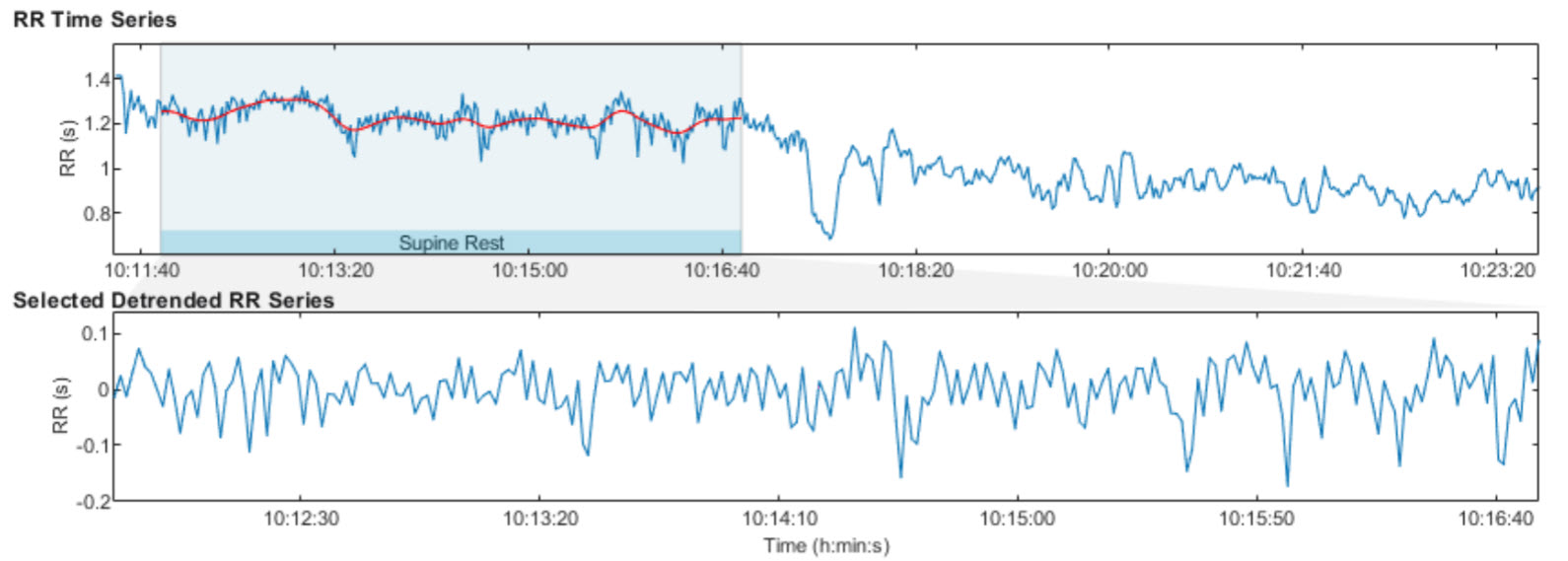
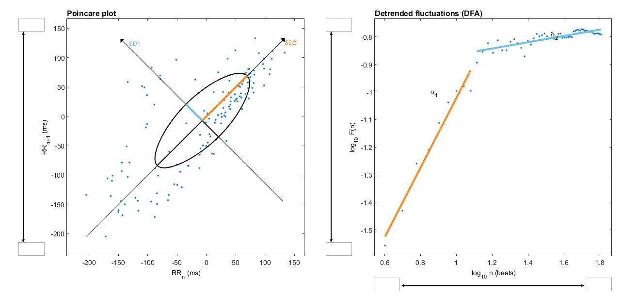
Nonlinearity describes a relationship between variables that cannot be plotted as a straight line. In HRV analysis, this means that the heart rate responds to physiological inputs in ways that are disproportionate, interactive, and context-dependent rather than following simple proportional rules. The graphic below from a 2-minute sample illustrates two common nonlinear displays: a Poincaré plot and a detrended fluctuation analysis plot.

Nonlinear Metrics in Clinical Context

This section covers what nonlinear measurements reveal about cardiovascular regulation, how they relate to the time-domain and frequency-domain indices you already use, and the important limitations clinicians should keep in mind. Nonlinear measurements quantify the unpredictability of a time series, which reflects the complexity of the regulatory mechanisms controlling heart rate. These indices correlate with specific frequency-domain and time-domain measurements when the same underlying physiological processes generate them.

While stressors and disorders like diabetes can depress nonlinear metrics, elevated values do not always signal health. In post-myocardial infarction (post-MI) patients, for example, increased nonlinear HRV is an independent risk factor for mortality (Stein et al., 2005). This distinction is critical for practitioners working with cardiac rehabilitation patients in hospital or VA settings: the same metric can mean recovery in one client and risk in another.

Karemaker (2020) cautioned that HRV entropy measures have yielded few practical applications and are not consistently superior to time- and frequency-domain measurements:

Comparisons between more classical statistical- or frequency analysis derived- and entropy-derived measures do, however, not always favor the newer ones (Zhang et al., 2013). This may, partly, be due to the fact that in many applications, entropy-measurements require rather long recordings before reaching a stable value. In critical situations this is a serious drawback. However, when the requirement of more time and more data points it is not an issue, entropy analysis may be a viable option to dig deeper in the complexities of the heart rate signal at hand.

BCIA Blueprint Coverage

BCIA's HRV Biofeedback Blueprint does not cover nonlinear metrics. However, understanding these measurements gives you a more complete picture of the tools available in software like Kubios and helps you interpret the research literature when nonlinear indices appear in published findings. Whether you work in a VA hospital interpreting post-deployment stress data or in a sports performance clinic analyzing an athlete's recovery profile, you may encounter nonlinear values in your HRV software reports.

This unit covers Poincaré plots, S, SD1, SD2, SD1/SD2, Approximate Entropy (ApEn), Sample Entropy (SampEn), Multiscale Entropy (MSE), Detrended Fluctuation Analysis (DFA), α1 and α2, and Correlation Dimension.

🎧 Listen to the Full Chapter Lecture

Poincaré Plot Analysis Reveals Hidden Patterns

This section explains how Poincaré plots are constructed, what they reveal about beat-to-beat heart rate dynamics, and why they offer a unique clinical perspective that frequency-domain methods do not. A Poincaré plot (return map) is created by plotting every R-R interval against the immediately preceding interval, producing a scatterplot. If your client's heart beats at intervals of 800 ms, then 750 ms, then 820 ms, you would plot the point (800, 750), then (750, 820), and so on. The resulting cloud of points reveals patterns buried within the time series—a sequence of successive values—that are invisible in a simple line graph.

Unlike frequency-domain measurements, Poincaré plot analysis is insensitive to slow drifts and trends in R-R intervals (Behbahani et al., 2012). This makes it especially valuable in settings such as VA sleep labs or sports physiology clinics, where you want to visualize the overall shape and spread of heart rate variability without the influence of gradual signal shifts caused by posture changes, circadian rhythms, or progressive fatigue.

S, SD1, SD2, and SD1/SD2: Quantifying the Poincaré Plot

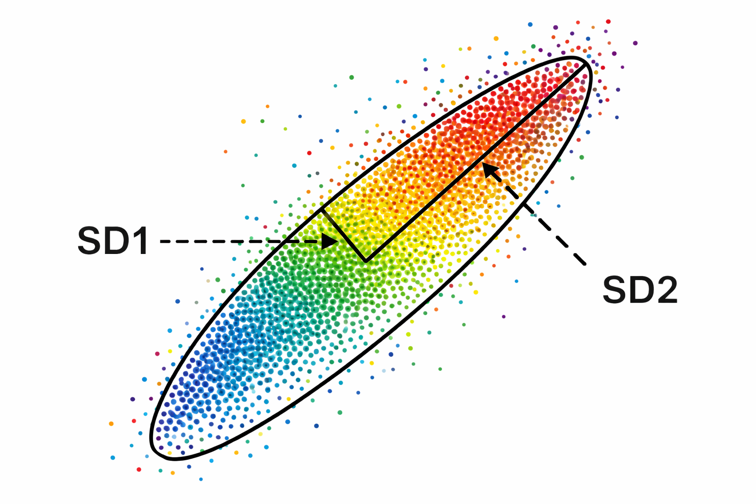
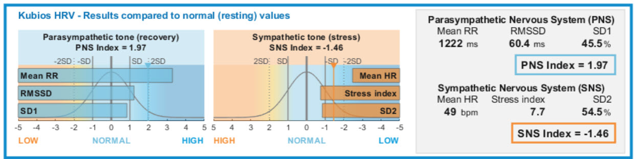
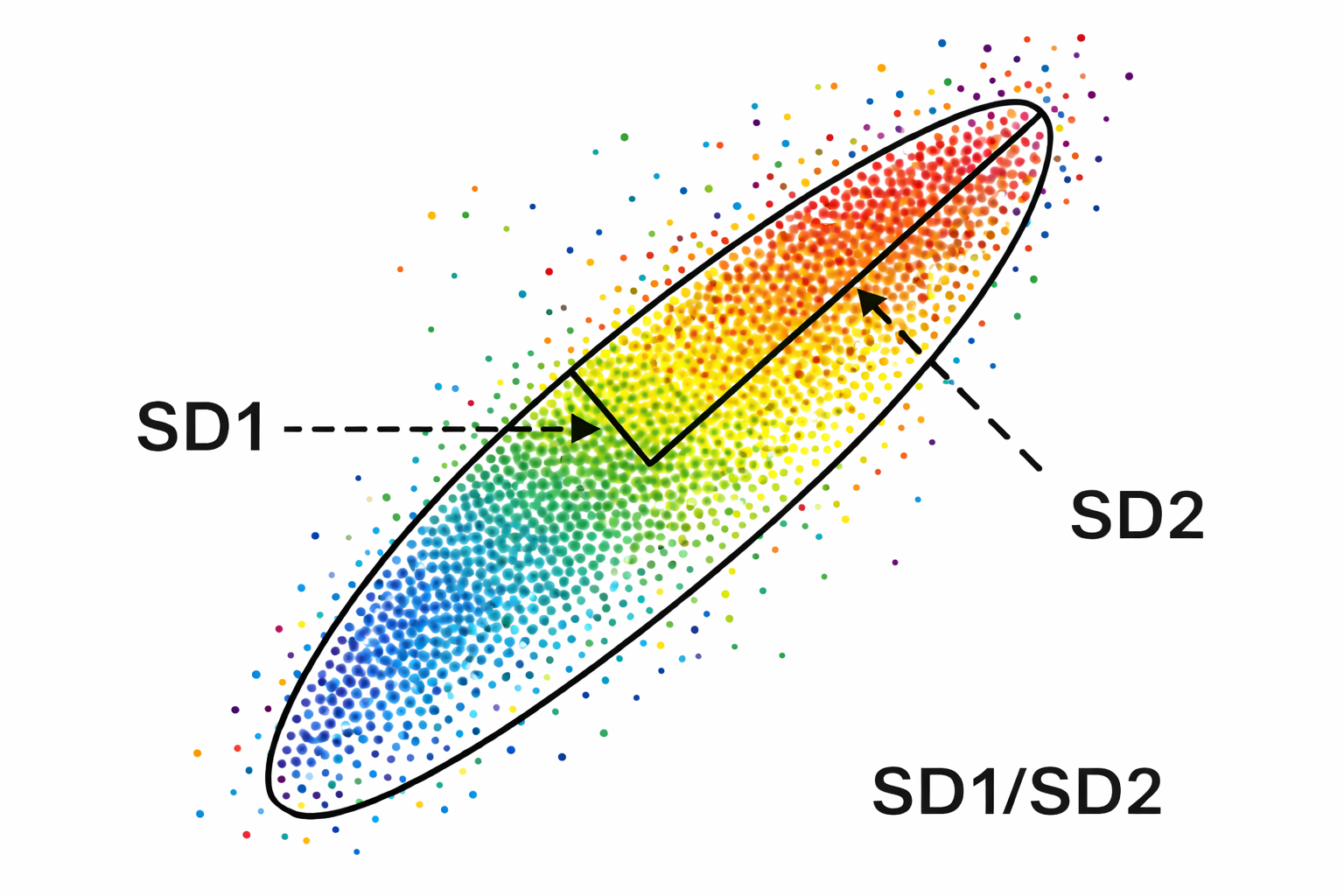
This section explains the four measurements derived from the Poincaré plot ellipse, what each one tells you physiologically, and how they connect to the time-domain and frequency-domain metrics you already use. We quantify a Poincaré plot by fitting an ellipse—a curve resembling a squashed circle—to the scattered points. This ellipse yields three primary nonlinear measurements: S, SD1, and SD2.

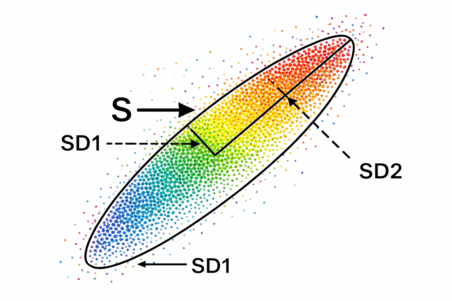
S measures the area of the ellipse, representing total HRV, and correlates with baroreceptor reflex sensitivity (BRS), LF and HF power, and RMSSD. SD1—the standard deviation (SD) of the distance of each point from the y = x axis—specifies the ellipse's width and measures short-term HRV in milliseconds. SD1 correlates with BRS and HF power. Importantly, SD1 is mathematically identical to the time-domain metric RMSSD, so when you see SD1 in a Kubios report, you are looking at the same short-term parasympathetic index you already know (Ciccone et al., 2017).

SD2—the standard deviation of each point from the y = x + average R-R interval—specifies the ellipse's length and captures both short- and long-term HRV in milliseconds. SD2 correlates with LF power and BRS (Brennan et al., 2001; Brennan et al., 2002; Tulppo et al., 1996; Tulppo et al., 1998). Kubios incorporates SD1 in its parasympathetic index and SD2 in its sympathetic index (Tarvainen & Niskanen, 2020). The data shown below were recorded from a healthy young man lying supine for 5 minutes.

SD1/SD2 Ratio and Autonomic Balance

The SD1/SD2 ratio measures the unpredictability of the R-R time series and is used to assess autonomic balance when the monitoring period is sufficiently long and sympathetic activation is present. SD1/SD2 is correlated with the LF/HF ratio, making it another window into the sympathovagal interplay that shapes your client's cardiovascular regulation (Behbahani et al., 2012; Guzik et al., 2012). All three Poincaré ellipse measures—S, SD1, and SD2—also correlate with baroreflex sensitivity, reinforcing the close link between nonlinear HRV and the body's blood pressure regulation loop.

One of the most practical additions to Poincaré interpretation is knowing where a client's values stand relative to healthy peers of the same age. A large population study by Voss et al. (2015) measured short-term resting HRV across a healthy adult cohort and reported age-decade means for SD1, SD2, and SD1/SD2 that clinicians can use as working reference bands. Because all three metrics decline substantially across the adult lifespan, comparing a value against an age-matched band is far more informative than applying a single adult threshold.

For SD1, which again is mathematically equivalent to RMSSD, typical resting means in the Voss et al. (2015) cohort run from roughly the high twenties to about 30 ms in adults aged 25 to 34, and fall to around the low teens in adults aged 65 to 74, with wide dispersion in every decade.

A practical way to use these figures is to treat an age decade's approximate mean plus or minus one standard deviation as a working clinical band, then prioritize within-person change over time. A 30-year-old whose resting SD1 sits persistently near the lower boundary of her decade band, combined with elevated resting heart rate and chronic insomnia, tells a coherent autonomic story that can anchor a sleep, recovery, and breathing intervention. Conversely, an endurance athlete whose SD1 rebounds toward his personal baseline after travel offers objective evidence of recovery, even when subjective fatigue has not yet cleared.

SD2 follows the same age-related trajectory. Voss et al. (2015) report mean SD2 values in the low-60 ms range for adults aged 25 to 34, declining to roughly the high-30 ms range for adults aged 65 to 74, again with substantial interindividual spread. Because SD2 captures both fast and slower oscillatory contributions across the recording window, it can remain informative even when SD1 is constrained by mild attentional stress or shallow breathing. Its limitation is sensitivity to slow drifts and posture shifts: even subtle trends in the RR series can inflate or distort SD2 unless the recording environment is controlled and appropriate detrending is applied (Magagnin et al., 2011).

The classic Task Force (1996) standardization guidelines are therefore even more important for SD2 than for SD1. A practical use case is cardiac rehabilitation: if an older patient's SD2 rises gradually across weeks of supervised activity and sleep consolidation while symptoms and blood pressure simultaneously improve, that convergence supports a genuine restoration of cardiovascular flexibility rather than a simple placebo response.

For the SD1/SD2 ratio, Voss et al. (2015) report typical mean values in roughly the mid-0.4 to about 0.5 range in younger adults, declining toward the mid-0.3 range in older adults, with broad dispersion throughout. Because the ratio compresses Poincaré geometry into a single shape descriptor, it can highlight pattern shifts that SD1 or SD2 alone might miss.

Two clients can share the same SD2 while carrying different SD1 values, and the ratio makes that asymmetry immediately visible. Its limitation is interpretive instability when either component approaches its lower distribution limit, because small denominators can produce misleading swings (Magagnin et al., 2011).

In performance settings, the ratio provides useful context for tactical athletes under operational stress. A practitioner whose client reports feeling "wired but tired" after several consecutive night shifts might find that SD2 remains moderate while SD1 and the SD1/SD2 ratio have both collapsed, pointing toward diminished short-term vagal modulation under accumulated sleep debt rather than simply elevated sympathetic drive. The intervention target becomes recovery scheduling and downregulation practice, not more training load.

Approximate Entropy: Measuring Signal Regularity

This section introduces entropy-based measures of HRV, beginning with approximate entropy and explaining how it quantifies the regularity and predictability of the heartbeat signal. Approximate entropy (ApEn) measures the regularity and complexity of a time series. It was specifically designed for brief, real-world recordings in which some noise may be present and makes no assumptions about the underlying system dynamics (Kuusela, 2013).

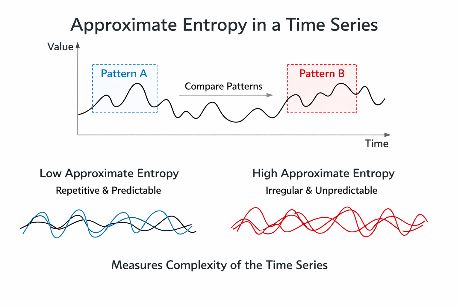
When applied to HRV data, large ApEn values indicate low predictability of fluctuations in successive R-R intervals, while small ApEn values mean the signal is regular and easy to anticipate (Beckers et al., 2001; Tarvainen & Niskanen, 2020). Think of ApEn as a measure of how "surprised" you would be by each successive heartbeat interval: a high ApEn means the next interval is hard to guess, while a low ApEn means the pattern is repetitive. In clinical practice, a very low ApEn in a cardiac patient may suggest that the heart's regulatory mechanisms have lost their normal adaptive complexity.

Sample Entropy: A Less Biased Alternative

Sample entropy (SampEn) was designed to provide a less biased and more reliable measure of signal regularity and complexity than ApEn (Richman & Moorman, 2000). Where ApEn can produce slightly inflated values due to the way it counts matching patterns, SampEn corrects this statistical artifact. SampEn values are more stable than ApEn for the same participant over successive days, making it a more dependable tracking metric for longitudinal monitoring (Richman & Moorman, 2000).

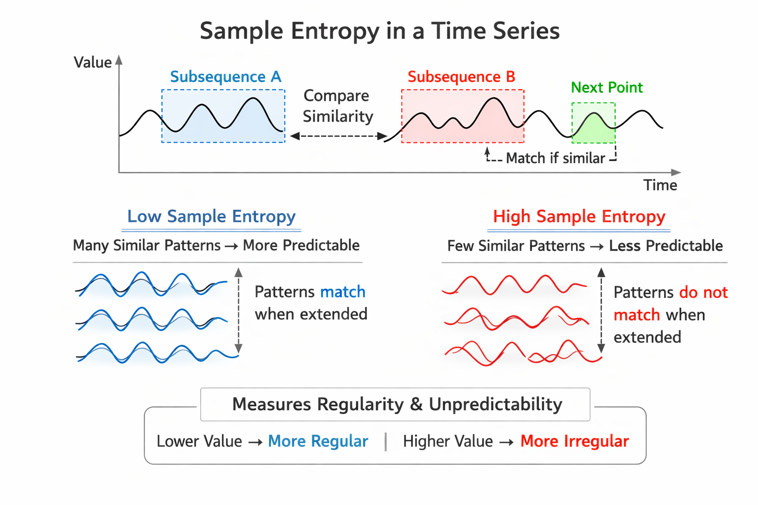
SampEn values are interpreted and used like ApEn but can be calculated from a much shorter time series of fewer than 200 values (Kuusela, 2013). This practical advantage makes SampEn particularly useful in clinical settings—such as busy VA outpatient clinics or pre-competition athlete assessments—where long recording sessions are not feasible. When you need a quick entropy estimate from a short recording, SampEn is the better choice.

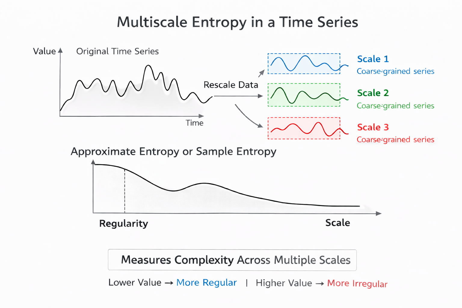
Multiscale Entropy: Looking at Multiple Time Scales

Multiscale Entropy (MSE) extends entropy analysis by using a resampling procedure to increase the number of data points in a time series, allowing researchers to detect slower fluctuations that simpler entropy methods might miss (Costa et al., 2002, 2005). While ApEn and SampEn analyze the signal at a single scale, MSE examines complexity across multiple time scales simultaneously—from beat-to-beat variation up through slower rhythms spanning minutes or hours.

This multi-resolution view makes MSE especially valuable for research into conditions like congestive heart failure or age-related autonomic decline, where the loss of complexity may only become apparent at longer time scales.

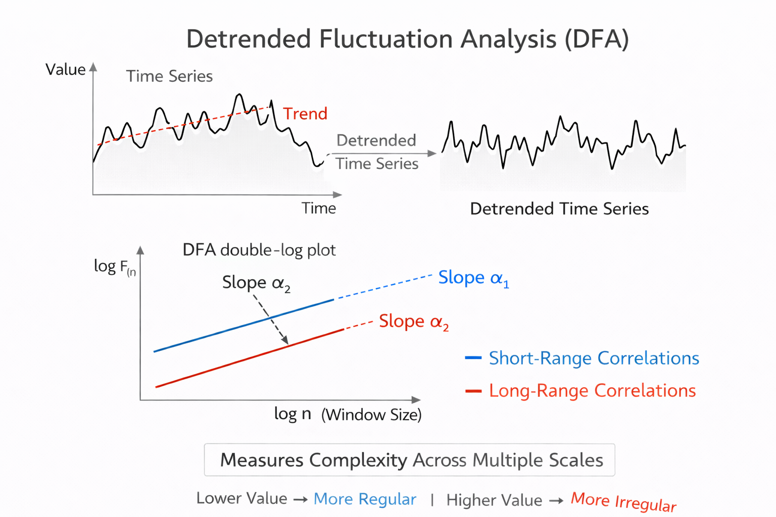
Detrended Fluctuation Analysis Extracts Correlations Across Time Scales

This section explains how detrended fluctuation analysis works, what its two output slopes represent physiologically, and why this method requires longer recordings than most clinical sessions provide. Detrended fluctuation analysis (DFA) extracts the correlations between successive R-R intervals over different time scales. It produces two key outputs: slope α1, which represents short-term fluctuations, and slope α2, which describes long-term fluctuations.

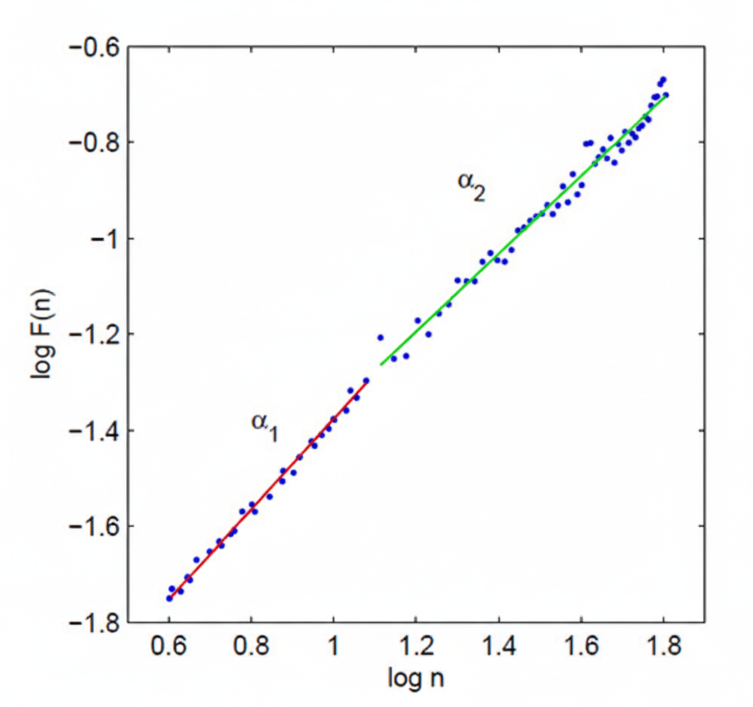
The short-term correlations captured by α1 primarily reflect the baroreceptor reflex—the rapid blood pressure regulation loop that adjusts heart rate on a beat-to-beat basis. The long-term correlations captured by α2 reflect broader regulatory mechanisms that limit the overall range of beat-to-beat fluctuation across hours. Because DFA is designed to analyze time series spanning several hours of data, it is best suited for 24-hour ambulatory recordings rather than the brief 5-minute sessions common in biofeedback practice (Kuusela, 2013).

In summary, DFA offers a window into how the heart's regulatory systems operate across very different time horizons. The α1 slope connects to the fast parasympathetic reflexes you target in HRV biofeedback, while α2 reveals the slower regulatory dynamics that shape cardiovascular health over hours and days. Understanding both slopes helps you interpret Kubios reports that include DFA results alongside your standard time-domain and frequency-domain metrics.

Age-stratified reference values for DFA α1 are available from the Voss et al. (2015) cohort, which used short-term resting recordings comparable to what most clinicians can reproduce in practice. Typical mean α1 values rise with age, from around 0.9 in adults aged 25 to 34 to roughly 1.1 in adults aged 65 to 74, with wide dispersion in each decade. This counterintuitive pattern reflects age-related changes in autonomic correlation structure rather than simply more variability, and it underscores why DFA α1 must be interpreted longitudinally and against age-appropriate reference bands rather than against a single population cutoff.

Clinically, the most defensible use is tracking change within the same person over time. If a patient with metabolic syndrome begins an aerobic training and sleep program, and DFA α1 drifts toward that individual's own prior healthier baseline while blood pressure, glucose control, and fatigue simultaneously improve, that convergence provides evidence of improved regulatory dynamics rather than a single noisy HRV value on one day (Shaffer & Ginsberg, 2017).

In performance settings, DFA α1 has attracted growing interest as a potential marker of exercise intensity domains when computed in short moving windows during exercise rather than from resting recordings (Rogers et al., 2022). This application rests on the observation that the fractal correlation structure of RR intervals shifts in characteristic ways across training zones, potentially offering a noninvasive intensity anchor. However, this use case requires tight control over data quality and consistent algorithm settings, because DFA α1 is notably sensitive to artifact correction strategies in ambulatory and exercise contexts (Rogers et al., 2021). If your practice includes exercise physiology, treat DFA α1 as a training intensity adjunct rather than a replacement for lactate, ventilatory, or pace-based anchors, and verify that correction methods and algorithm settings are held stable across devices and sessions.

Compression Entropy: Quantifying Pattern Richness in the RR Series

Entropy methods aim to quantify the unpredictability and pattern richness of a time series, and the repeated finding that reduced complexity accompanies both aging and illness is one of the most robust themes in physiologic systems research (Lipsitz & Goldberger, 1992; Richman & Moorman, 2000). Compression entropy (Hc3,3) operationalizes this idea by asking how compressible the RR interval sequence is. The underlying logic is elegant: if a lossless compression algorithm can represent the series in very few bits, the series contains mostly repeated patterns and is therefore stereotyped. If the algorithm must use many bits, the series is rich with non-repeating structure. More compressible sequences reflect more stereotyped cardiac dynamics in this framework, while less compressible ones signal the kind of pattern diversity associated with healthy, flexible autonomic regulation.

Voss et al. (2015) included Hc3,3 in their large healthy cohort study alongside the Poincaré and DFA metrics described above, which makes it one of the few entropy-family measures with age-stratified reference values from a well-characterized resting dataset. Mean Hc3,3 is higher in younger adults and declines across the adult decades, moving roughly from the high 0.7 range in the youngest age groups to around the low 0.6 range in adults aged 65 to 74, with meaningful dispersion at every decade. This trajectory is consistent with the broader physiologic complexity literature (Henriques et al., 2020; Lipsitz & Goldberger, 1992).

The strength of a compression-based approach is that it can be less tied to a single parametric definition of irregularity than some classical entropy choices, while still tracking the clinical intuition that healthy physiology does not repeat itself mechanically. Its limitation is that it is less familiar to most clinicians than ApEn or SampEn, and like other entropy-family measures it can be biased by nonstationarity, filtering choices, and artifact editing decisions (Henriques et al., 2020; Magagnin et al., 2011).

Nonstationarity refers to time-varying changes in the mean or variance of the RR series, such as those caused by postural shifts, emotional responses, or breathing irregularities during recording.

Because Hc3,3 is sensitive to these influences, the same standardization principles that apply to SD1 and DFA α1 apply here as well: consistent posture, caffeine and nicotine restrictions, and stable breathing instructions reduce noise that would otherwise contaminate the complexity estimate (Task Force of the European Society of Cardiology and the North American Society of Pacing and Electrophysiology, 1996). For recording duration, treat Hc3,3 like other short-term nonlinear indices: a 5-minute resting segment is workable for repeated measurement when preprocessing is careful and conditions are stable (Voss et al., 2015).

The most defensible clinical use of Hc3,3 is as a longitudinal indicator of pattern diversity that complements the variance-based Poincaré metrics. When SD1 and Hc3,3 move together in the same direction across a treatment program, the two independent perspectives strengthen the inference. When they diverge, the divergence itself is informative.

In a paced breathing and activity-pacing program for chronic pain patients, for example, resting SD1 might improve as vagal modulation increases during training sessions while Hc3,3 remains low, indicating that the patient is gaining cardiovascular responsiveness within the clinic but has not yet recovered the day-to-day adaptability that reflects genuine systemic improvement. That pattern often marks the right moment to introduce generalization tasks, such as brief breathing resets during real-world stressors, rather than extending the length of in-clinic breathing sessions.

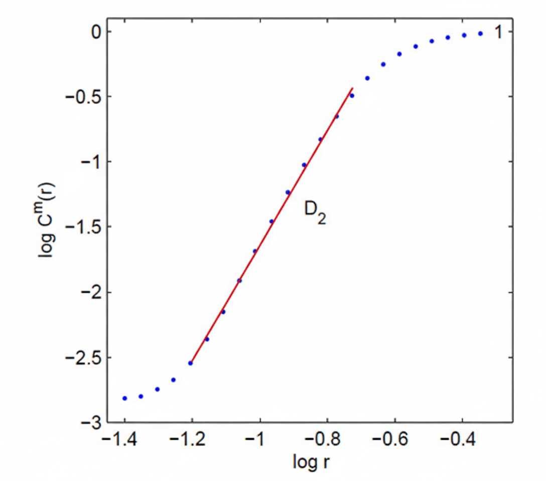
Correlation Dimension: Estimating System Complexity

This section introduces the correlation dimension as a measure of cardiovascular system complexity and explains the concept of attractors that underlies it. The correlation dimension estimates the minimum number of variables required to construct a model of the system's dynamics. The more variables needed to predict the time series, the greater the system's complexity—and the more regulatory mechanisms are actively shaping the heartbeat pattern.

An attractor is a set of values toward which a variable in a dynamic system converges over time.

Think of it as a marble rolling in a bowl: no matter where you release it, the marble eventually settles toward the bottom. In cardiovascular physiology, attractors represent the characteristic states that heart rate dynamics naturally gravitate toward under stable conditions. The correlation dimension measures the attractor dimension—which can be an integer or a fractal number—of these converging patterns (Kuusela, 2013). A fractal dimension suggests that the system's behavior is more complex than any simple geometric shape can capture.

How Long Must You Record? Minimum Periods for Each Nonlinear Metric

One of the most practically important and frequently overlooked questions in nonlinear HRV analysis is how many heartbeats, and how many minutes of recording, each metric actually requires before it yields a trustworthy number. The answer is more nuanced than any single value can capture, because researchers have identified two distinct thresholds that matter in different clinical and research situations. The first is the bare computational minimum: the fewest R-peaks needed to produce a numerical output at all. The second, and more clinically important, is the consistency threshold: the shortest recording that yields values statistically consistent with a longer, more reliable reference segment (Chou et al., 2021).

Both thresholds are reported here as a range of beats and approximate minutes at a resting heart rate of 60 bpm, alongside the conventional short-term standard of 5 minutes established by the Task Force (1996).

Because time in minutes depends entirely on heart rate, the most rigorous way to express these requirements is in R-peaks or NN intervals rather than clock time. The conversion is straightforward: required time in minutes equals the required number of beats divided by the heart rate in beats per minute (Chou et al., 2021). A client resting at 75 bpm will accumulate 1,000 NN intervals in about 13 minutes; a well-trained athlete resting at 45 bpm will need closer to 22 minutes to reach the same count. Always calculate your minimum recording time from your individual client's actual heart rate rather than a textbook average.

SD1: The Shortest Acceptable Recording

Because SD1 is mathematically identical to RMSSD, it inherits RMSSD's relatively modest data requirements (Ciccone et al., 2017). Both metrics reflect rapid, beat-to-beat parasympathetic modulation, which means meaningful signal exists even in brief recordings. Chou et al. (2021) found that SD1 reaches consistency with longer reference recordings at a minimum of approximately 60 NN intervals, equivalent to roughly 1 minute at 60 bpm. This is the lowest consistency threshold of any nonlinear metric reviewed in that study and reflects the fact that the parasympathetic fluctuations driving SD1 occur on the same short time scale as the recording window itself.

Shaffer and Ginsberg (2017) confirmed this finding in a review of pediatric normative data, demonstrating that SD1, alongside RMSSD, pNN50, and HF power, can be reliably measured from 1-minute recordings. Shaffer et al. (2019) applied a more conservative criterion of Pearson r greater than or equal to 0.90 against a 5-minute reference and found that a 90-second segment met this threshold, establishing it as a validated ultra-short-term surrogate. The conventional short-term standard endorsed by the Task Force (1996) remains 5 minutes, corresponding to approximately 300 NN intervals at 60 bpm. The acceptable recording range for SD1 therefore spans from roughly 60 intervals (1 minute) to 300 intervals (5 minutes), with 90 seconds representing the validated ultra-short-term minimum and 5 minutes the established clinical standard.

SD2: Longer Recordings Capture the Full Picture

SD2 tells a very different story from SD1. Where SD1 reflects fast parasympathetic fluctuations, SD2 captures both short- and long-term variability by measuring the spread of the Poincaré plot ellipse along the line of identity. Because it incorporates the slower LF-band rhythms that unfold over periods of 7 to 25 seconds, SD2 demands a longer recording to sample enough complete oscillation cycles to produce a stable estimate (Shaffer & Ginsberg, 2017). Chou et al. (2021) found that SD2 requires at least 1,000 NN intervals to reach consistency with a longer reference recording, corresponding to approximately 16.7 minutes at 60 bpm.

Shaffer et al. (2019) identified a 90-second segment as a surrogate for SD2 by the Pearson correlation criterion, but the same research tradition acknowledges that 5-minute recordings are required for SD2 to carry clinical meaning, because the LF-band rhythms that drive it need sufficient time to complete enough cycles for reliable estimation (Shaffer & Ginsberg, 2017).

The Task Force (1996) 5-minute standard is therefore the defensible clinical minimum for SD2. The acceptable range for SD2 spans from 300 intervals (5 minutes) for clinical short-term use to 1,000 intervals (about 17 minutes) for maximum consistency, with 24-hour recordings as the gold standard when sympathetic contributions to SD2 are the focus of assessment.

SD1/SD2: Interpreting Autonomic Balance Requires Adequate Time

The SD1/SD2 ratio indexes the unpredictability of the R-R time series and estimates autonomic balance, but only when the monitoring period is long enough and the conditions are appropriate for sympathetic engagement (Shaffer & Ginsberg, 2017). Because the ratio incorporates SD2 in the denominator, it inherits SD2's sensitivity to recording length. Chou et al. (2021) found that the SD1/SD2 ratio requires at least 1,000 NN intervals, or approximately 16.7 minutes, to reach consistency with longer reference recordings. Unlike SD1, no validated ultra-short-term surrogate has been established for the ratio as a whole (Shaffer & Ginsberg, 2017).

The Task Force (1996) 5-minute standard applies as the accepted short-term floor, giving an acceptable range of 300 intervals (5 minutes) at the lower end to 1,000 intervals (about 17 minutes) at the consistency threshold. For interpretations that depend on detecting sympathetic contributions to the ratio, 24-hour ambulatory recording is preferred because sympathetic influences unfold over much longer time scales than a brief resting session can capture (Shaffer & Ginsberg, 2017).

Approximate Entropy: Designed for Short Series, but Not Infinitely So

Pincus (1991) designed ApEn specifically to work with short, noisy time series that offer no guarantees about the underlying system dynamics. In the original publication, meaningful ApEn values were obtained from as few as 50 to 100 data points, equivalent to under 2 minutes at 60 bpm. This was a deliberate design choice: ApEn was intended for clinical situations where long recordings are not feasible, and it makes no assumptions about the dynamics of the underlying system (Shaffer & Ginsberg, 2017). For HRV specifically, large ApEn values indicate low predictability of successive R-R fluctuations, while small values signal a regular and easily anticipated pattern (Beckers et al., 2001; Tarvainen & Niskanen, 2020).

Despite this theoretical lower bound, practical reliability improves substantially with more data. Yentes et al. (2013) demonstrated that at least 200 data points are recommended for ApEn estimates to become reasonably stable, and that both ApEn and SampEn are sensitive to data length in ways that can distort comparisons across studies if recording durations differ.

Chou et al. (2021) found that ApEn requires approximately 1,000 NN intervals to reach consistency with longer reference recordings, corresponding to about 16.7 minutes at 60 bpm. The Task Force (1996) 5-minute standard applies as the conventional short-term minimum. No validated ultra-short-term surrogate has been established for ApEn distinct from the 5-minute standard (Shaffer & Ginsberg, 2017).

The practical range for ApEn therefore runs from 50 to 100 intervals (under 2 minutes) for bare-minimum computation (Pincus, 1991), through 200 intervals for basic reliability (Yentes et al., 2013), to 300 intervals (5 minutes) as the clinical standard (Task Force, 1996), and approximately 1,000 intervals (about 17 minutes) for full consistency with longer recordings (Chou et al., 2021).

Sample Entropy: More Stable at Short Lengths, Still Demanding for Full Consistency

SampEn improves on ApEn by eliminating self-comparison when counting template matches, which removes the systematic bias that inflates ApEn at short data lengths (Richman & Moorman, 2000). This statistical advantage makes SampEn more stable than ApEn for the same participant across successive days and allows it to be computed from fewer than 200 NN intervals while still producing interpretable values (Kuusela, 2013; Richman & Moorman, 2000). Yentes et al. (2013) recommended at least 200 data points for reliable SampEn estimation, though SampEn retains more validity below that threshold than ApEn does.

Shaffer et al. (2019) found that a 180-second (3-minute) segment met the conservative criterion of r greater than or equal to 0.90 against a 5-minute reference, establishing it as a validated ultra-short-term surrogate. Chou et al. (2021) extended this analysis and found that consistency with longer recordings requires approximately 1,000 NN intervals, or about 16.7 minutes.

The acceptable range for SampEn therefore spans from fewer than 200 intervals for basic computation, through 180 seconds as the ultra-short-term validated minimum (Shaffer et al., 2019), to 300 intervals (5 minutes) as the conventional standard (Task Force, 1996), and approximately 1,000 intervals (about 17 minutes) for full statistical consistency (Chou et al., 2021).

DFA Alpha-1: Reliable in Shorter Windows, Best With More Data

DFA alpha-1 quantifies short-term fractal correlations by analyzing fluctuations over beat ranges of approximately 4 to 16 beats (Peng et al., 1995). Because it captures correlations that manifest within a relatively brief span of the time series, alpha-1 is more forgiving of short recording lengths than most other nonlinear metrics. Fractal behavior as revealed by DFA alpha-1 can be reliably observed in RR intervals spanning 5 minutes or less (Shaffer & Ginsberg, 2017). Shaffer et al. (2019) found that a 120-second (2-minute) segment, corresponding to roughly 120 NN intervals at 60 bpm, met the r greater than or equal to 0.90 consistency criterion against the 5-minute reference.

Chou et al. (2021) applied a stricter consistency analysis and found that DFA-derived measures require at least 1,500 NN intervals, approximately 25 minutes at 60 bpm, for full statistical agreement with longer recordings. This gap between the ultra-short-term surrogate threshold of 120 seconds and the full consistency threshold of 25 minutes reflects the difference between a metric functioning as a useful clinical proxy and providing a fully stable statistical estimate.

The acceptable range for DFA alpha-1 therefore spans from 120 seconds as the validated ultra-short-term minimum (Shaffer et al., 2019), through 300 intervals (5 minutes) as the conventional short-term standard (Task Force, 1996), to 1,500 intervals (about 25 minutes) for maximum consistency (Chou et al., 2021).

DFA Alpha-2: Long-Range Correlations Demand Long Recordings

DFA alpha-2 describes long-term fractal scaling by analyzing fluctuations over beat ranges of approximately 17 to 64 beats (Peng et al., 1995). Because it captures correlations that only emerge across longer stretches of the time series, alpha-2 is substantially more data-hungry than alpha-1. Shaffer et al. (2019) found that a 180-second (3-minute) segment met the r greater than or equal to 0.90 criterion against the 5-minute reference, establishing the validated ultra-short-term surrogate threshold. Chou et al. (2021) found that full consistency with longer recordings requires at least 1,500 NN intervals, equivalent to approximately 25 minutes at 60 bpm.

The same caveat that applies to SD2 applies here: the long-range regulatory mechanisms that alpha-2 reflects unfold over hours, and the metric's clinical and prognostic value has been established primarily from 24-hour ambulatory recordings (Kuusela, 2013; Task Force, 1996).

The acceptable range for DFA alpha-2 runs from 180 seconds as the validated ultra-short-term surrogate (Shaffer et al., 2019), through 300 intervals (5 minutes) as the conventional minimum (Task Force, 1996), to 1,500 intervals (about 25 minutes) for consistency (Chou et al., 2021), with 24-hour recordings as the preferred standard whenever the physiological interpretation of long-range autonomic regulation is the primary goal.

Correlation Dimension: The Most Data-Hungry Metric of All

The correlation dimension (D2) estimates the minimum number of variables required to model the dynamic system generating the heartbeat time series, and it is by far the most demanding nonlinear HRV metric in terms of recording length (Kuusela, 2013). The mathematical basis for this demand comes from embedding theory: reliable estimation of D2 requires a number of data points that grows exponentially with the embedding dimension d.

A widely cited practical heuristic holds that approximately 10 raised to the power d data points are needed, where d is the embedding dimension used in the analysis (Chou et al., 2021; Grassberger & Procaccia, 1983). At the commonly used embedding dimension of 6, this means roughly 1,000,000 beats, equivalent to approximately 277 hours at 60 bpm, a requirement that no practical clinical recording can meet.

Shaffer et al. (2019) confirmed the clinical reality of this constraint: no ultra-short-term recording below 5 minutes produced a valid surrogate for D2 when compared against a 5-minute reference. Meaningful D2 estimation therefore requires substantially longer recordings than the standard 5-minute session (Shaffer & Ginsberg, 2017).

Research employing D2 for prognostic purposes uses 24-hour ambulatory monitoring as the practical standard, and even those recordings fall well short of what the mathematics would ideally demand (Chou et al., 2021; Grassberger & Procaccia, 1983). The correlation dimension has no validated short-term clinical minimum: treat any D2 output from a brief recording as a rough indicator rather than a reliable estimate.

Multiscale Entropy: Recording Demands Scale With the Scales You Analyze

MSE extends SampEn across multiple time scales by progressively coarse-graining the original NN interval series, averaging adjacent values within windows of increasing length to create new, slower time series at each scale (Costa et al., 2002). This coarse-graining procedure is mathematically elegant but has a direct and unavoidable consequence for recording requirements: at scale factor tau, the length of the available time series shrinks to approximately N divided by tau, where N is the total number of intervals in the original recording (Wu et al., 2013).

At the higher scale factors used in full MSE analysis, this reduction can bring the available data points well below the minimum needed for stable SampEn estimation, causing the entropy values at those scales to become unreliable.

Wu et al. (2013) derived a practical guideline for this problem: for SampEn at a given scale to be largely free of length effects, the coarse-grained series at that scale should contain at least approximately 750 data points. This means the original recording must contain at least 750 times the maximum scale factor analyzed. For a maximum scale of 5, the minimum original recording is 3,750 NN intervals, roughly 62 minutes at 60 bpm. For full-range analysis up to scale 20, the minimum becomes 15,000 NN intervals, approximately 250 minutes (about 4.2 hours) at 60 bpm (Wu et al., 2013).

The original MSE methodology employed by Costa et al. (2002) used time series of approximately 30,000 data points, corresponding to roughly 500 minutes (about 8.3 hours) at 60 bpm, drawn from 24-hour Holter recordings to ensure stability at all scale factors. Chou et al. (2021) found that MSE reaches consistency with longer reference recordings at a minimum of approximately 1,000 NN intervals (about 16.7 minutes), though this applies only to low-scale output.

The acceptable recording range for MSE therefore spans from roughly 1,000 intervals (about 17 minutes) for low-scale results (Chou et al., 2021), through 15,000 intervals (about 250 minutes) for analysis up to scale 20 (Wu et al., 2013), to the gold-standard 24-hour recording used in the foundational literature (Costa et al., 2002).

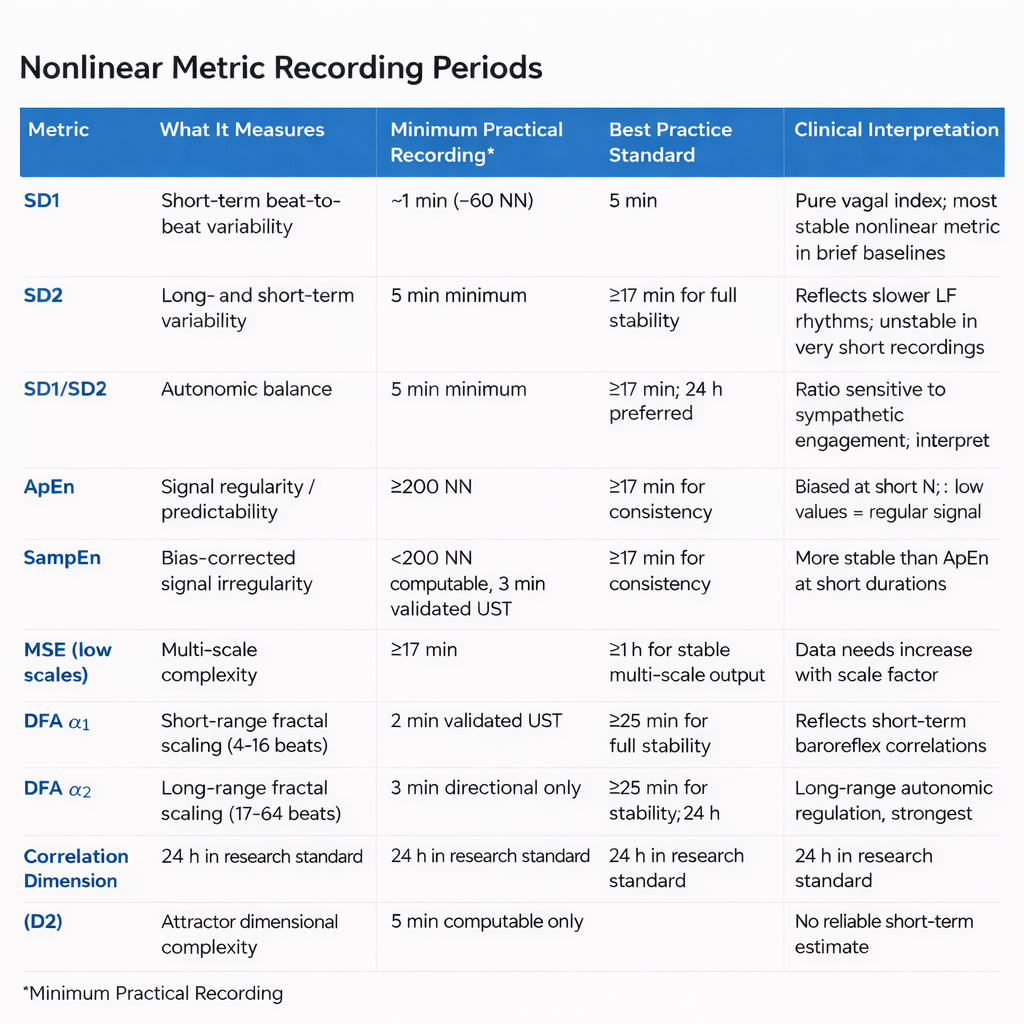
Minimum Recording Periods: Summary Table

The table below consolidates the recording requirements reported above. Each row reports the full acceptable range for that metric, from the briefest computationally viable segment at the low end to the standard most appropriate for clinical and research use at the high end. All beat counts represent NN intervals at a resting heart rate of 60 bpm; divide by the client's actual heart rate to convert to minutes (Chou et al., 2021). The validated ultra-short-term (UST) minimum is the shortest segment confirmed by Shaffer et al. (2019) to correlate at r ≥ 0.90 with a 5-minute reference. The consistency threshold is the minimum reported by Chou et al. (2021) for reliable agreement with a longer reference recording.

Interpreting Nonlinear HRV: Context Is Everything

Is Increased Nonlinearity Always Desirable?

If nonlinear measurements of HRV are reduced in diseases like diabetes, is increased nonlinearity always desirable? The answer is no—it depends on which physiological processes generate the nonlinearity. While increased nonlinear HRV values could signal improved health in a diabetic client with better glucose control, those same elevated values could signal a greater risk of death in a post-MI patient (Stein et al., 2005). This distinction is one of the most important clinical lessons in this entire unit.

For practitioners in cardiac rehabilitation, VA hospitals, or intensive care settings, this means that nonlinear HRV values cannot be interpreted in isolation. You must always consider the client's diagnosis, medical history, and current treatment context before deciding whether a change in nonlinear metrics represents progress or a warning sign.

How Professionals Should Use Nonlinear Metrics in Practice

The single most important principle for using nonlinear HRV metrics in applied settings is to standardize your acquisition with the same rigor you would apply to a laboratory assay. Use the same posture, time-of-day window, caffeine and nicotine rules, and breathing instructions every time a client is assessed. This is especially critical for nonlinear measures, which are more sensitive to preprocessing choices, recording conditions, and nonstationarity than most time-domain metrics (Shaffer & Ginsberg, 2017; Task Force of the European Society of Cardiology and the North American Society of Pacing and Electrophysiology, 1996). The professional skill is less about knowing how to compute a DFA α1 or an Hc3,3 and more about computing them comparably across time and across people, so that a change in value reflects a change in physiology rather than a change in protocol.

Preprocessing transparency is equally essential. Inspect the raw RR series before analysis, document every artifact correction decision, and be cautious with aggressive filtering, because heavy filtering can reshape nonlinear structure in ways that alter entropy and fractal estimates without altering the time-domain metrics that might otherwise flag the problem (Magagnin et al., 2011; Tarvainen et al., 2014). When slow trends are present in the recording, such as a gradual rise in heart rate across the session, apply an appropriate detrending step and report it, because slow drifts can contaminate both spectral and nonlinear estimates (Tarvainen et al., 2002). Kubios HRV offers built-in options for artifact correction and detrending, and using them consistently and documenting those settings is part of professional practice.

A practical starting point is to treat nonlinear metrics as second opinions on autonomic regulation rather than standalone diagnostic tests. Reviews consistently group the most clinically workable nonlinear indices into Poincaré plot geometry, fractal scaling, and entropy or complexity measures (Henriques et al., 2020; Shaffer & Ginsberg, 2017). Use age-decade reference values from studies like Voss et al. (2015) as a reality check, but treat within-person trajectories as primary. A healthy 65-year-old can sit at the upper end of her decade band, and a deconditioned 30-year-old can sit near the lower end, so the clinically meaningful question is whether the metric moves in response to your intervention and whether that movement aligns with symptom change. This is where nonlinear metrics genuinely earn their place: they can reveal regained adaptability even when average variability levels remain modest.

For clinical care, the convergence of multiple signals creates the strongest evidence. If SD1 rises, DFA α1 shifts toward a more fractal pattern, and Hc3,3 increases simultaneously while a patient reports fewer headaches, better sleep, and lower pain ratings across a 10-week program, those converging signals support a coherent story of improved autonomic regulation. If only one metric moves while the others stay flat, the clinician's job is to ask whether a real change occurred at a specific timescale, whether the metric is picking up a recording artifact, or whether the intervention has simply not yet produced broad enough change to register across methods.

Finally, avoid the common trap of equating higher with better. For variance-based indices like SD1 and SD2, unusually high values can reflect cardiac arrhythmia or poor beat detection rather than exceptional fitness. For fractal and entropy measures, deviations from the typical range can be context-dependent in ways that require clinical judgment. The professional stance is to treat nonlinear HRV as evidence about the quality of cardiovascular control, evidence that becomes clinically meaningful only when it is reproducible, appropriately contextualized within the client's history, and tied to outcomes you can observe directly.

Assignment

Now that you have completed this module, explain the difference between linear and nonlinear relationships. When might greater nonlinear HRV values be worrisome?

Glossary

References

Beckers, F., Ramaekers, D., & Aubert, A. E. (2001). Approximate entropy of heart rate variability: Validation of methods and application in heart failure. Cardiovascular Engineering: An International Journal, 1(4), 177-182. https://doi.org/10.1023/A:1015212328405

Behbahani, S., Dabanloo, N. J., & Nasrabadi, A. M. (2012). Ictal heart rate variability assessment with focus on secondary generalized and complex partial epileptic seizures. Advances in Bioresearch, 4(1), 50-58.

Brennan, M., Palaniswami, M., & Kamen, P. (2001). Do existing measures of Poincaré plot geometry reflect nonlinear features of heart rate variability? IEEE Transactions on Biomedical Engineering, 48(11), 1342-1347. https://doi.org/10.1109/10.959330

Brennan, M., Palaniswami, M., & Kamen, P. (2002). Poincaré plot interpretation using a physiological model of HRV based on a network of oscillators. American Journal of Physiology-Heart and Circulatory Physiology, 283, H1873-H1886. https://doi.org/10.1152/ajpheart.00405.2000

Carrasco, S., Gaitán, R., González, R., & Yánez, O. (2001). Correlation among Poincaré plot indexes and time and frequency domain measures of heart rate variability. Journal of Medical Engineering & Technology, 25(6), 240-248. https://doi.org/10.1080/03091900110086651

Chou, E.-F., Khine, M., Lockhart, T., & Soangra, R. (2021). Effects of ECG data length on heart rate variability among young healthy adults. Sensors, 21(18), 6286. https://doi.org/10.3390/s21186286. PMID: 34577492

Ciccone, A. B., Siedlik, J. A., Wecht, J. M., Deckert, J. A., Nguyen, N. D., & Weir, J. P. (2017). Reminder: RMSSD and SD1 are identical heart rate variability metrics. Muscle & Nerve, 56(4), 674-678. https://doi.org/10.1002/mus.25573

Costa, M., Goldberger, A. L., & Peng, C. K. (2002). Multiscale entropy analysis of complex physiologic time series. Physical Review Letters, 89, 068102. https://doi.org/10.1103/physrevlett.89.068102

Costa, M., Goldberger, A. L., & Peng, C. K. (2005). Multiscale entropy analysis of biological signals. Physical Review E, 71, 021906. https://doi.org/10.1103/physreve.71.021906

Guzik, P., Piskorski, J., Krauze, T., & Wysocki, H. (2012). The influence of changing respiratory rate on HRV is portrayed by descriptors of Poincaré analysis. Unpublished manuscript obtained from ResearchGate.

Grassberger, P., & Procaccia, I. (1983). Characterization of strange attractors. Physical Review Letters, 50(5), 346-349. https://doi.org/10.1103/PhysRevLett.50.346

Henriques, T., Ribeiro, M., Teixeira, A., Castro, L., Antunes, L., & Costa Santos, C. (2020). Nonlinear methods most applied to heart rate time series: A review. Entropy, 22(3), 309. https://doi.org/10.3390/e22030309

Huikuri, H. V., Mäkikallio, T. H., Raatikainen, P., Perkiömäki, J., Castellanos, A., & Myerburg, R. J. (2003). Prediction of sudden cardiac death: Appraisal of the studies and methods assessing the risk of sudden arrhythmic death. Circulation, 108(1), 110-115. https://doi.org/10.1161/01.cir.0000077519.18416.43

Karemaker, J. M. (2020). Interpretation of heart rate variability: The art of looking through a keyhole. Frontiers in Neuroscience, 14, 609570. https://doi.org/10.3389/fnins.2020.609570

Kuusela, K. (2013). Methodological aspects of heart rate variability analysis. In M. V. Kamath, M. A. Watanabe, & A. R. M. Upton (Eds.), Heart rate variability (HRV) signal analysis. CRC Press.

Lake, D. E., Richman, J. S., Griffin, M. P., & Moorman, J. R. (2002). Sample entropy analysis of neonatal heart rate variability. American Journal of Physiology-Regulatory, Integrative and Comparative Physiology, 283, R789-R797. https://doi.org/10.1152/ajpregu.00069.2002

Lippman, N., Stein, K. M., & Lerman, B. B. (1994). Comparison of methods for removal of ectopy in measurement of heart rate variability. American Journal of Physiology, 267(1 Pt 2), H411-H418. https://doi.org/10.1152/ajpheart.1994.267.1.h411

Lipsitz, L. A., & Goldberger, A. L. (1992). Loss of complexity and aging: Potential applications of fractals and chaos theory to senescence. JAMA, 267(13), 1806-1809. https://doi.org/10.1001/jama.1992.03480130122036

Magagnin, V., Bassani, T., Bari, V., Turiel, M., Maestri, R., Pinna, G. D., & Porta, A. (2011). Non-stationarities significantly distort short-term spectral, symbolic, and entropy heart rate variability indices. Physiological Measurement, 32(11), 1775-1786. https://doi.org/10.1088/0967-3334/32/11/S05

Peng, C.-K., Havlin, S., Stanley, H. E., & Goldberger, A. L. (1995). Quantification of scaling exponents and crossover phenomena in nonstationary heartbeat time series. Chaos: An Interdisciplinary Journal of Nonlinear Science, 5(1), 82-87. https://doi.org/10.1063/1.166141. PMID: 11538314

Perkiomaki, J. S., Zareba, W., Badilini, F., & Moss, A. J. (2002). Influence of atropine on fractal and complexity measures of heart rate variability. Annals of Noninvasive Electrocardiology, 7(4), 326-330. https://doi.org/10.1111/j.1542-474x.2002.tb00181.x

Pincus, S. M. (1991). Approximate entropy as a measure of system complexity. Proceedings of the National Academy of Sciences of the United States of America, 88(6), 2297-2301. https://doi.org/10.1073/pnas.88.6.2297. PMID: 2041994

Richman, J. S., & Moorman, J. R. (2000). Physiological time-series analysis using approximate entropy and sample entropy. American Journal of Physiology-Heart and Circulatory Physiology, 278(6), H2039-H2049. https://doi.org/10.1152/ajpheart.2000.278.6.h2039. PMID: 10843903

Rogers, B., Giles, D., Draper, N., Hoos, O., & Gronwald, T. (2021). Influence of artifact correction methods on the relationship between detrended fluctuation analysis alpha one and running intensity. International Journal of Environmental Research and Public Health, 18(4), 2016. https://doi.org/10.3390/ijerph18042016

Rogers, B., Peçanha, T., & Gronwald, T. (2022). Detrended fluctuation analysis of heart rate variability in endurance exercise: A systematic review. Frontiers in Physiology, 13, 1016447. https://doi.org/10.3389/fphys.2022.1016447

Schrödinger, E. (1944). What is life? The physical aspect of the living cell. Cambridge University Press.

Shaffer, F., & Ginsberg, J. P. (2017). An overview of heart rate variability metrics and norms. Frontiers in Public Health, 5, 258. https://doi.org/10.3389/fpubh.2017.00258. PMID: 29034226

Shaffer, F., Shearman, S., Meehan, Z., Gravett, N., & Urban, H. (2019). The promise of ultra-short-term (UST) heart rate variability measurements: A comparison of Pearson product-moment correlation coefficient and limits of agreement (LoA) concurrent validity criteria. In D. Moss & F. Shaffer (Eds.), Physiological recording technology and applications in biofeedback and neurofeedback (pp. 214-220). Association for Applied Psychophysiology and Biofeedback.

Stein, P. K., Domitrovich, P. P., Huikuri, H. V., & Kleiger, R. E. (2005). Traditional and nonlinear heart rate variability are each independently associated with mortality after myocardial infarction. Journal of Cardiovascular Electrophysiology, 16(1), 13-20. https://doi.org/10.1046/j.1540-8167.2005.04358.x

Tarvainen, M. P., & Niskanen, J.-P. (2020). Kubios HRV version 3.4 user's guide. Kubios Oy.

Tarvainen, M. P., Niskanen, J. P., Lipponen, J. A., Ranta-aho, P. O., & Karjalainen, P. A. (2014). Kubios HRV: Heart rate variability analysis software. Computer Methods and Programs in Biomedicine, 113(1), 210-220. https://doi.org/10.1016/j.cmpb.2013.07.024

Tarvainen, M. P., Ranta-aho, P. O., & Karjalainen, P. A. (2002). An advanced detrending method with application to HRV analysis. IEEE Transactions on Biomedical Engineering, 49(2), 172-175. https://doi.org/10.1109/10.979357

Task Force of the European Society of Cardiology and the North American Society of Pacing and Electrophysiology. (1996). Heart rate variability: Standards of measurement, physiological interpretation, and clinical use. Circulation, 93, 1043-1065.

Tulppo, M. P., Makikallio, T. H., Seppanen, T., Laukkanen, R. T., & Huikuri, H. V. (1998). Vagal modulation of heart rate during exercise: Effects of age and physical fitness. American Journal of Physiology, 274, H424-H429. https://doi.org/10.1152/ajpheart.1998.274.2.h424

Tulppo, M. P., Makikallio, T. H., Takala, T. E., Seppanen, T., & Huikuri, H. V. (1996). Quantitative beat-to-beat analysis of heart rate dynamics during exercise. American Journal of Physiology, 271, H244-H252. https://doi.org/10.1152/ajpheart.1996.271.1.h244

Voss, A., Schroeder, R., Heitmann, A., Peters, A., & Perz, S. (2015). Short-term heart rate variability: Influence of gender and age in healthy subjects. PLOS ONE, 10(3), e0118308. https://doi.org/10.1371/journal.pone.0118308

Wu, S.-D., Wu, C.-W., Lin, S.-G., Wang, C.-C., & Lee, K.-Y. (2013). Time series analysis using composite multiscale entropy. Entropy, 15(3), 1069-1084. https://doi.org/10.3390/e15031069

Yentes, J. M., Hunt, N., Schmid, K. K., Kaipust, J. P., McGrath, D., & Stergiou, N. (2013). The appropriate use of approximate entropy and sample entropy with short data sets. Annals of Biomedical Engineering, 41(2), 349-365. https://doi.org/10.1007/s10439-012-0668-3. PMID: 23064819

Zhang, Y., de Peuter, O. R., Kamphuisen, P. W., & Karemaker, J. M. (2013). Search for HRV-parameters that detect a sympathetic shift in heart failure patients on β-blocker treatment. Frontiers in Physiology, 4, 81. https://doi.org/10.3389/fphys.2013.00081