
The Use of Different EEG Montages for Waveform Analysis
What You Will Learn in This Chapter
Two clinicians can look at the same recording and see different brains. Not because one of them is careless, but because they chose different montages. The electrodes on the scalp collect voltage; the montage decides what each channel is compared against, and that decision determines which activity survives to the screen and which gets subtracted away. Change the reference and posterior alpha can appear in a frontal trace that never generated it.
This unit works through the montage configurations you will use in clinical and research EEG: referential or monopolar, sequential or bipolar with its longitudinal, transverse, and circular variants, average reference, linked ears, Laplacian, common average, source derivation, and Cz reference. For each, you will study how it is constructed, what it reveals, how it handles artifact, and where it misleads. We begin with the differential amplifier and common mode rejection, because every montage depends on them, and we close with the American Clinical Neurophysiology Society's best-practice recommendations.
IQCB Blueprint Coverage: This unit addresses The Use of Different EEG Montages for Waveform Analysis (IV.F) within EEG (IV), and supports Standards of EEG Acquisition Procedures (IV.D).
Learning Objectives
After completing this section, you will be able to:
Explain how a differential amplifier produces a channel and how common mode rejection suppresses shared signals.
Define derivation, montage, and reference contamination, and explain how the three relate.
Compare the referential, sequential, average reference, linked ears, Laplacian, common average, source derivation, and Cz reference montages.
Identify phase reversals in a longitudinal bipolar montage and explain what they localize.
Explain the edge effect in Laplacian and source derivation montages and why it limits peripheral electrodes.
Select an appropriate montage for a given clinical question and justify the choice.
State the ACNS Guideline 3 recommendations for montage construction and display.
Listen to the Full-Length Lecture
Using a Limited Number of Electrodes
This section examines the practical question of how many EEG channels you need for effective assessment and training. Peer-reviewed evidence indicates that increasing the number of electrodes improves spatial sampling and the accuracy with which independent sources can be separated from artifact; Lau et al. (2012), for example, found that source-separation accuracy in mobile EEG improved as channel count rose. It is important to distinguish that finding from the further claim that more channels produce better clinical or performance outcomes in neurofeedback, which has not been established by controlled trials. Although some practitioners conduct assessment and training with a single channel, multi-channel methods have become increasingly accessible as costs have decreased.
A full 19-channel EEG assessment, for example, not only provides amplitude and frequency data from every site in the 10-20 system but also enables computation of metrics such as coherence (the consistency of the common frequency content between two sites), phase (the timing relationship between signals at different sites) and co-modulation (the similarity in magnitude changes between two sites).
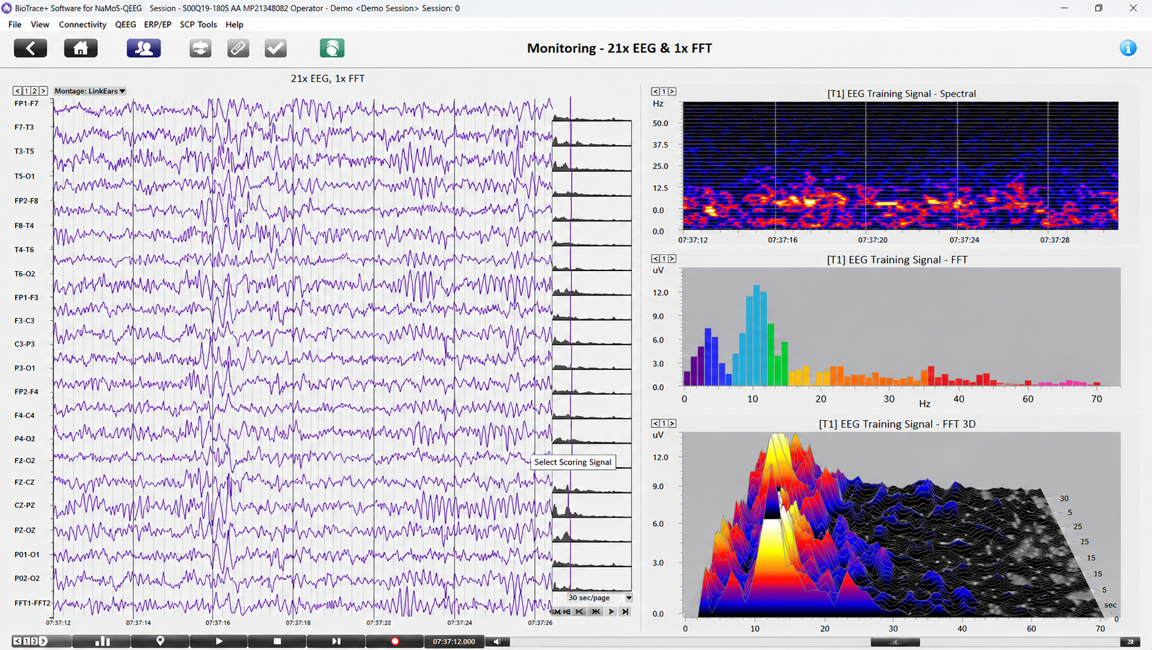
Raw Tracings and Multiple Spectral Displays from BioTrace - Mind Media
These connectivity metrics describe statistical relationships between the signals recorded at two sites, which are commonly interpreted as indexing communication between brain regions; a single channel cannot yield them at all. Because volume conduction and the choice of reference can inflate apparent connectivity, these measures require careful artifacting and cautious interpretation. Multi-channel data are particularly beneficial for complex symptom profiles like those associated with Autism Spectrum Disorders, epilepsy, and traumatic brain injury (Thompson & Thompson, 2015).
Graphic © Chaikom/Shutterstock.com.
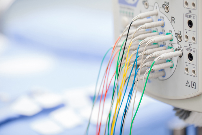
A channel is an EEG amplifier output resulting from scalp electrical activity detected through three electrode connections: the active (positive) electrode, placed over a known EEG generator like Cz; the reference (negative) electrode, which may be located on the scalp, earlobe, or mastoid; and the ground electrode, also typically placed on an earlobe or mastoid (Thompson & Thompson, 2015). Terminology varies across textbooks and manufacturers. The two signal electrodes are more precisely described as input 1 (noninverting, +) and input 2 (inverting, −), and the third electrode is more precisely described as the amplifier's common or ground connection, which establishes the reference potential for the amplifier but contributes no signal of its own. The word "reference" is unfortunately used for both input 2 and this common connection, so read each source carefully.
Electrically, the two signal inputs are balanced and interchangeable; reversing them does not change the magnitude of the recorded difference, but it does invert the polarity of the displayed waveform. Some neurofeedback data acquisition systems nonetheless require that a specific sensor be designated the "reference," as in a linked-ears reference.
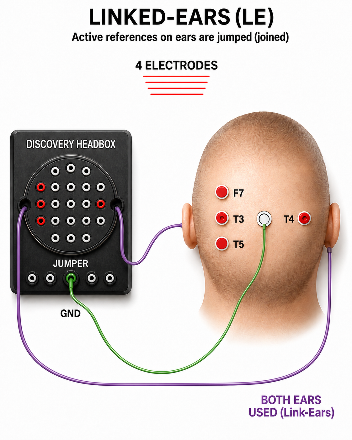
The graphic was adapted from John Demos' BCIA-recommended Getting Started with EEG Neurofeedback (2nd ed.). The ear references are connected as a common reference for the four active electrodes (F7, T3, T4, and T5).
A derivation is the assignment of two electrodes to an amplifier's inputs 1 and 2. For example, Fp1 to O2 means that Fp1 is placed in input 1 and O2 in input 2. A montage groups multiple derivations together to record EEG activity across several channels simultaneously (Thomas, 2007). Most modern digital amplifiers acquire every input relative to a single hardware reference—commonly Cz, FCz, CPz, or a mastoid, depending on the system—so montage changes are performed in software rather than by manually switching electrode connections.
All montages compare EEG activity between one or more pairs of electrode sites.
Montage Options and Their Consequences
Referential (Monopolar) Montage
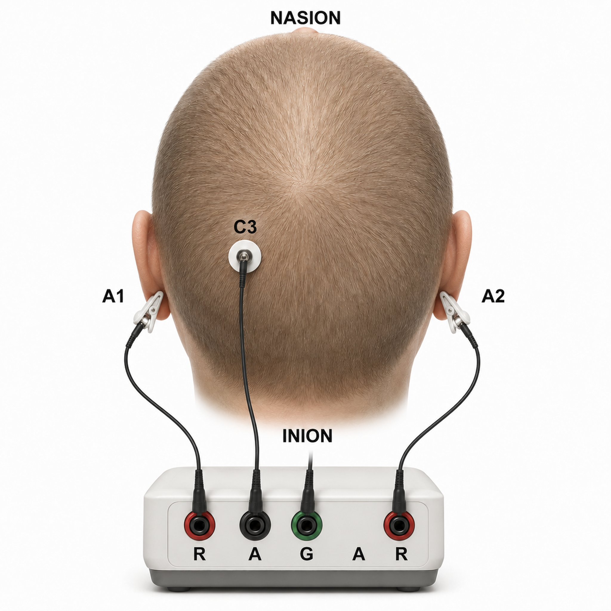
A referential (monopolar) montage places one active electrode (A) on the scalp and a "neutral" reference (R) and ground (G) on the ear or mastoid. This montage assumes that the EEG activity displayed on your screen represents the active (+) site, because the reference (−) site is presumed to be electrically quiet. That assumption is never fully satisfied: no scalp or ear site is truly inactive, so the displayed waveform always reflects the difference between the two sites. The differential amplifier amplifies the difference between its two inputs while rejecting the portion common to both, a property called common-mode rejection, which attenuates noise and artifacts shared by both sites.
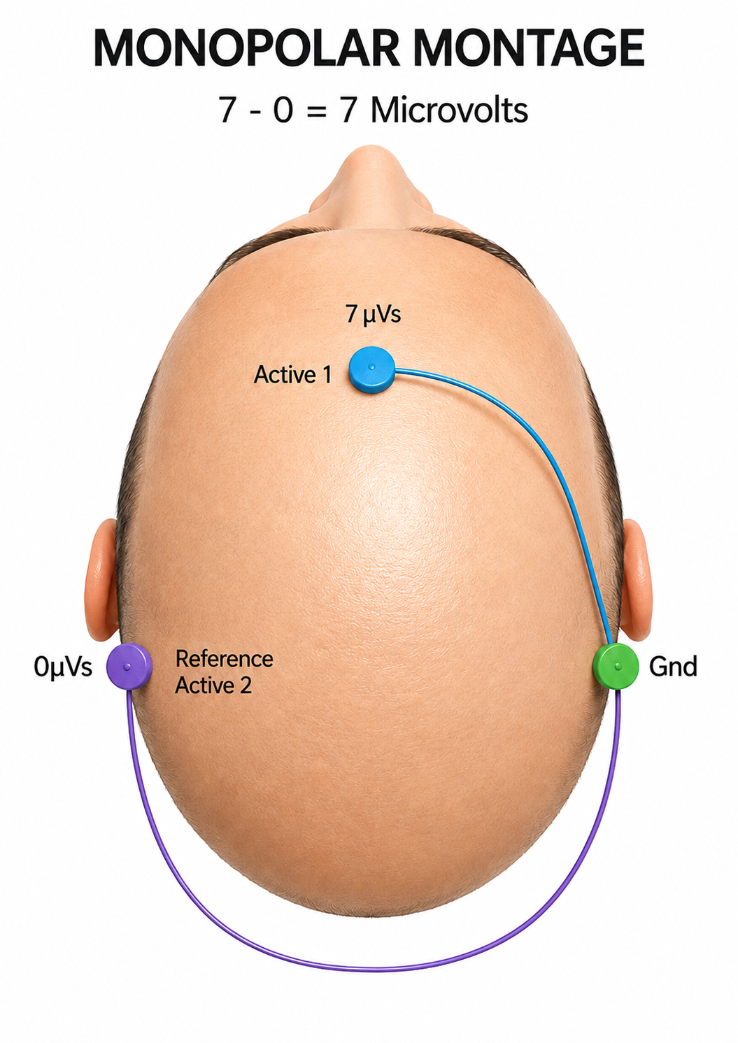
We adapted this graphic from John Demos' BCIA-recommended Getting Started with EEG Neurofeedback (2nd ed.). The active electrode "sees" 7 microvolts while the reference "sees" 0 microvolts, so the amplifier outputs their difference of 7 microvolts. This idealized example assumes a perfectly inactive reference.
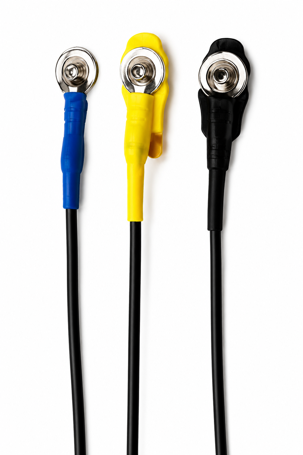
In the photograph below, the blue cable would be used for the active electrode, the yellow cable with an ear clip for reference, and the black cable with an ear clip for the ground.
However, this montage is vulnerable to artifacts from the contraction of facial muscles (Demos, 2019). The ear reference can also introduce reference contamination, where EEG signals picked up by the ear electrode are added to other channels through the differential amplifier, since the amplifier retains anything that differs between the active and reference inputs. This commonly results in alpha activity from posterior sources close to the ear appearing in channels where it does not belong.
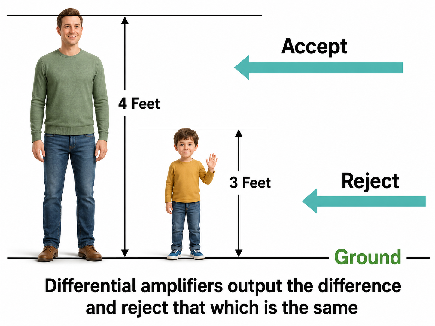
We adapted this graphic from John Demos' BCIA-recommended Getting Started with EEG Neurofeedback (2nd ed.). In this height analogy, a differential amplifier rejects the portion common to both inputs (e.g., 3 feet) and outputs only the difference (e.g., 4 feet). A single-ended amplifier outputs the entire value (e.g., 7 feet, artifact plus signal). The units here are illustrative only; actual EEG voltages are measured in microvolts.
Sequential (Bipolar) Montage
A sequential (bipolar) montage compares EEG activity between two scalp electrodes, both considered "active" sites, rather than referencing one to a presumed-neutral ear or mastoid. The positive (+) and negative (−) electrodes (often called "active" and "reference") are both attached to the scalp, while the ground (G) electrode is placed on the scalp, an earlobe, or over the mastoid process. Like the referential montage, this configuration detects the voltage difference between its two inputs, but now both inputs carry cerebral EEG signals.
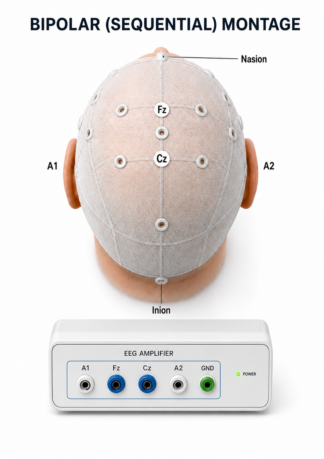
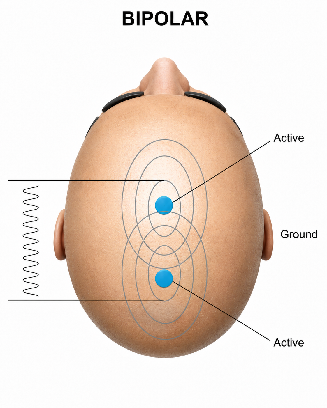
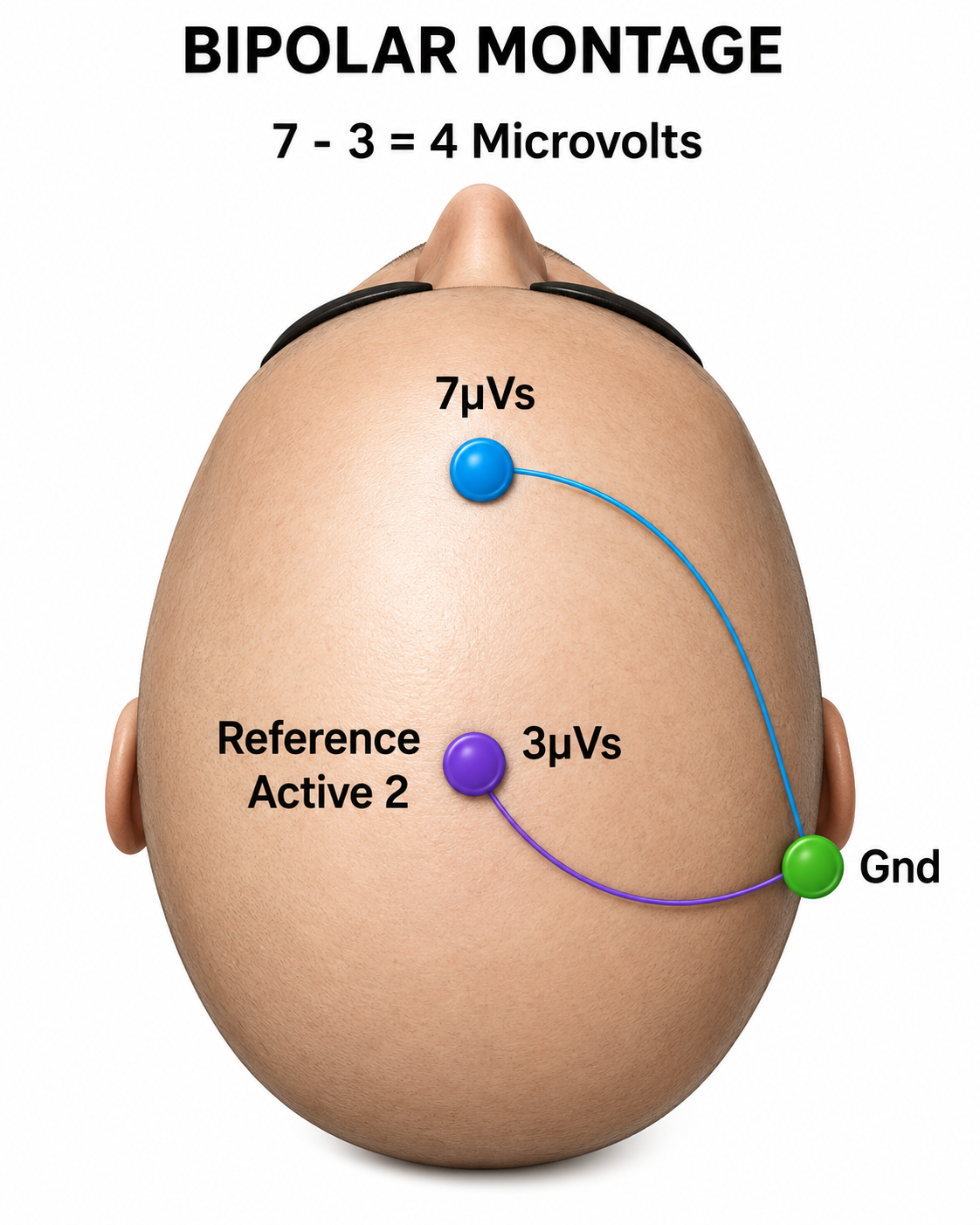
We adapted this graphic from John Demos' BCIA-recommended Getting Started with EEG Neurofeedback (2nd ed.). In the diagram on the right, the active "sees" 7 microvolts while the reference "sees" 3 microvolts. A differential amplifier subtracts these voltages, leaving 4 microvolts.
When 19 channels are used, this montage presents electrode pairs shown in sequence. Note that only the black cable for the ground has an ear clip in the photograph below. As a single channel, this montage does not localize EEG activity well because it shows only the difference between the A and R signals. However, when used as part of a 19-channel assessment, it excels at localizing EEG events related to epilepsy and can reduce artifacts when the A and R electrodes are relatively close together.
A sequential montage is frequently used in neurofeedback, where it trains the difference between EEG activity at the A and R electrodes. One important caveat: when training produces a change, it remains uncertain whether the change occurred at the A electrode, the R electrode, or both. The two signals are generally more similar when sensors are closer together and less similar when they are farther apart (e.g., Fp1-O2). When the two electrodes record nearly the same potential—as homologous frontopolar sites such as Fp1 and Fp2 often do—this montage may cancel genuine EEG activity along with the noise, a phenomenon sometimes called in-phase cancellation.
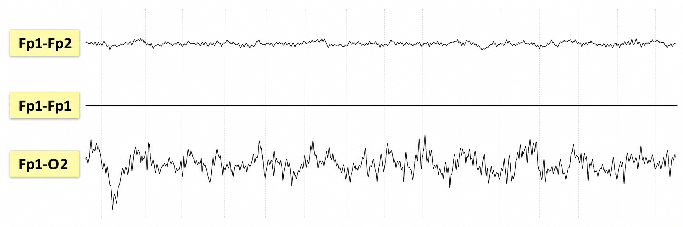
Graphic © John S. Anderson. Fp1–Fp2: low-amplitude, irregular mixed-frequency activity with no major frontal polar voltage difference. Fp1–Fp1: flat/isoelectric tracing, as expected because the same electrode is compared with itself. Fp1–O2: much higher-amplitude irregular slow activity, maximal in this wide anterior–posterior derivation; this suggests a large voltage gradient between Fp1 and O2.
Montages for 21 Recording Electrodes
All montages compare EEG activity between one or more pairs of electrode sites.
Listen to Lecture: Signal Acquisition (Montages)
This section examines the major montage configurations used in clinical EEG with 21 recording electrodes. The choice of montage does not alter the raw cortical electrical activity itself but rather filters, enhances, or diminishes specific aspects of it based on the spatial relationship between electrodes and the brain's dipolar sources, the electrical fields that produce opposing voltages detectable at the scalp. A montage defines how each EEG channel is constructed by determining which electrodes are compared to each other.
Broadly, montages fall into two categories. In a bipolar montage, each channel represents the voltage difference between two adjacent or anatomically aligned electrodes, emphasizing local voltage gradients. This configuration is especially useful for identifying focal abnormalities, such as epileptiform discharges, through phase reversals, points where waveform polarity inverts along a chain of electrodes, indicating the likely location of maximal voltage. The longitudinal bipolar ("double banana") montage arranges channels along the anterior-posterior axis, while the transverse montage organizes them across the coronal plane from left to right.
In contrast, a referential montage displays the voltage at each active electrode relative to a common reference point, which may be a single electrode, a pair of electrodes, or a mathematically computed value like the average of all electrodes. Referential montages are particularly suited for assessing global brain activity, hemispheric asymmetries, and background rhythms. Examples include the average reference, Cz reference, and linked ears montages. The Laplacian montage is often grouped with the referential montages because each electrode is compared to a computed value—a weighted average of its immediate neighbors—but it is more accurately described as a spatial filter, since it has no common reference site at all.
The sections that follow examine the structure, clinical utility, and interpretive implications of each montage. By understanding the distinction between bipolar and referential configurations, you can select the most appropriate montage for a given diagnostic question and use re-montaging, applying multiple montages to the same data set, for more comprehensive analysis.
Longitudinal Bipolar Montage
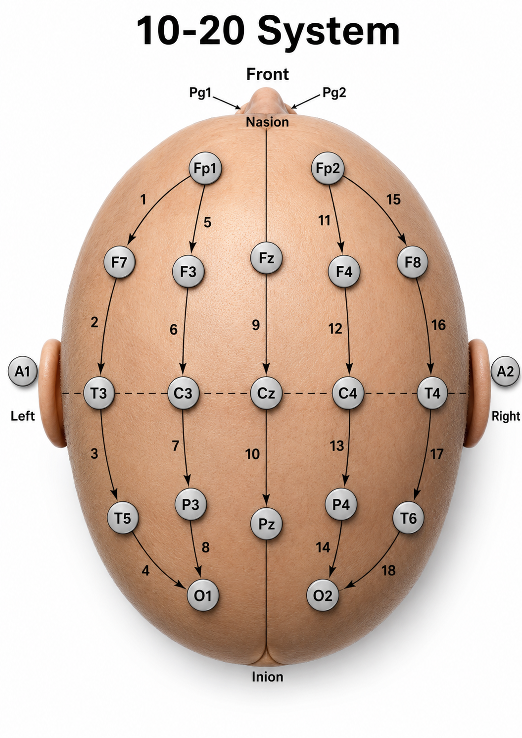
The longitudinal bipolar (double banana) montage is one of the most widely used configurations in clinical electroencephalography. It consists of bipolar derivations arranged in parallel chains, linking electrodes from the frontal to the occipital poles along the midline and lateral scalp. For example, one left-hemisphere chain includes the derivations Fp1-F3, F3-C3, C3-P3, and P3-O1, with a mirror chain on the right: Fp2-F4, F4-C4, C4-P4, and P4-O2.
Recording
The images below show the same sample of EEG with different montages.
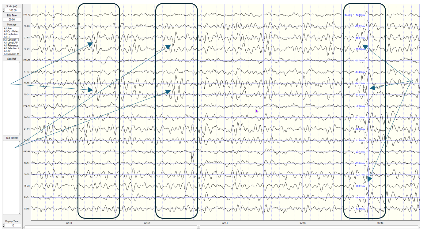
Longitudinal Bipolar Montage (Long BP) — Scale: 100 µV — 13-year-old male. The boxes mark sections of the recording where the phase reversals are clearest, and the arrows indicate the phase reversals themselves. This is a sequential montage—the longitudinal bipolar montage—in which a chain of electrode pairs is compared in order. Note that the first pairs, beginning with Fp1–F3 and followed by F3–C3, do not show the very high-amplitude 6 Hz activity (between 75 and 100 µV) that appears in the C3–P3 derivation and continues into the P3–O1 derivation. Observe that the waves in these two adjacent derivations point alternately toward and away from one another, indicating that the two are 180 degrees out of phase—that is, deflecting in opposite directions. This phase reversal locates the source of the high-amplitude activity beneath the electrode common to both derivations, in this case P3.
Below this, a second phase reversal appears between T3–T5 and T5–O1, localizing that source to T5. A similar but much lower-amplitude waveform is present at F3–C3 and F7–T3, reflecting a diminishing field in the derivations farther from the source.
Strengths
The primary strength of this montage is its capacity to reveal phase reversals, the inversion points of waveform polarity along the bipolar chain, which serve as a crucial diagnostic cue for localizing the maximum field of a focal discharge. This makes the montage particularly effective at detecting focal epileptiform activity organized along the sagittal plane (Niedermeyer & da Silva, 2005). The montage is also intuitive and standardized, which promotes consistent interpretation across clinical institutions.
Limitations
However, the longitudinal bipolar montage has notable limitations. Activity that is spatially generalized across adjacent electrode pairs may be attenuated or even canceled if it appears in phase across a chain. Activity oriented vertically or obliquely relative to the anteroposterior axis may also be poorly resolved due to the montage's directional bias. Additionally, this montage may be less sensitive to activity originating from deep cortical structures, such as mesial temporal regions.
Transverse Montage
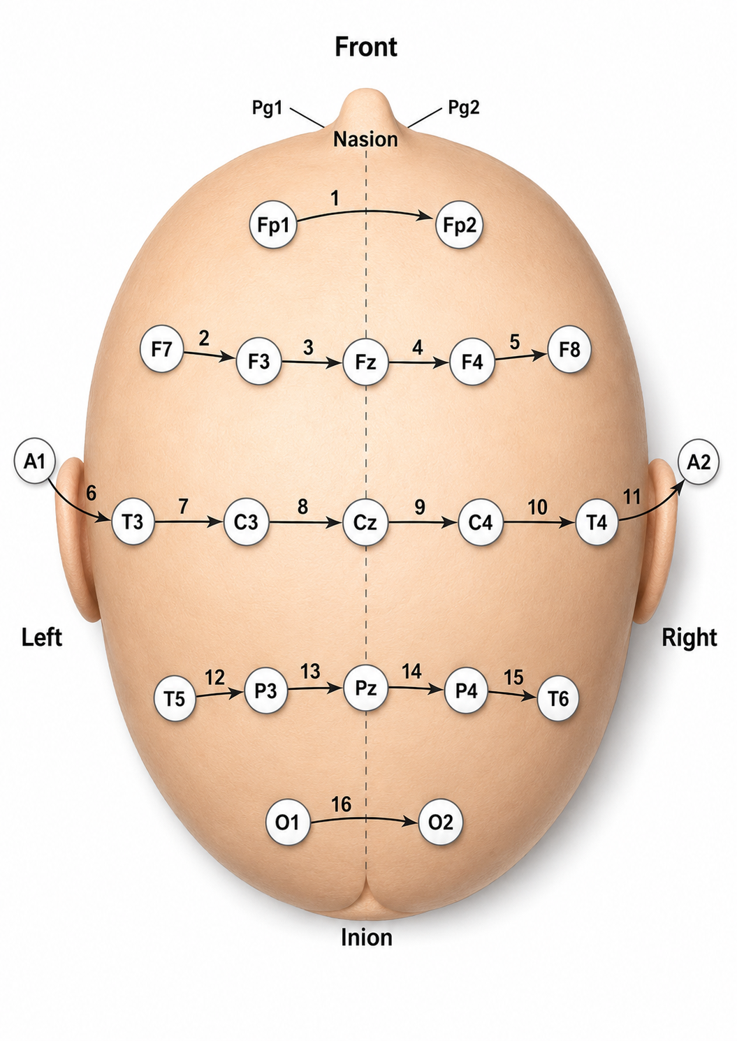
The transverse (coronal bipolar) montage links electrodes across the coronal plane, from one hemisphere to the other. A typical frontal chain might include F7-F3-Fz-F4-F8, followed by T3-C3-Cz-C4-T4 at the central level, and T5-P3-Pz-P4-T6 through the parietal and temporal regions. This left-to-right orientation complements the front-to-back view of the longitudinal bipolar montage.
Recording
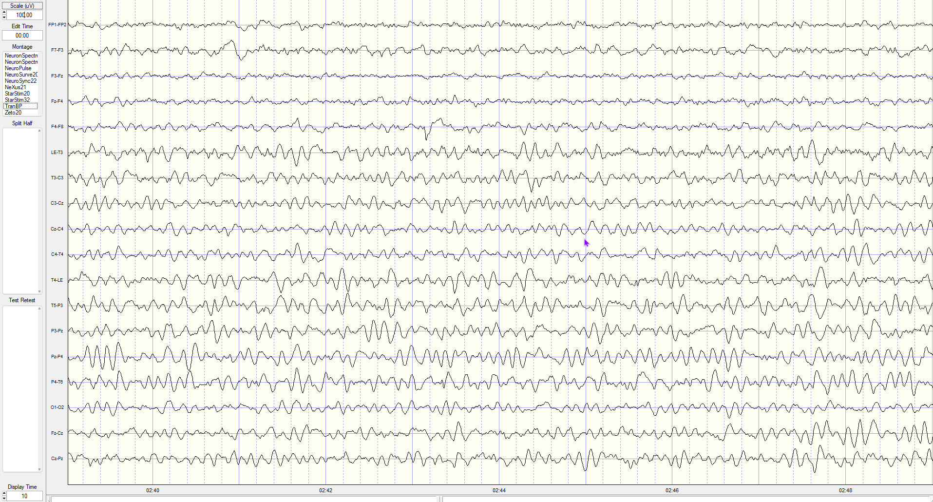
Transverse Bipolar Montage (Trans BP) — Here the phase reversals are less well defined, because this source is best revealed in the anterior–posterior derivations of the longitudinal bipolar montage. Overall power is also lower: each channel displays the difference between its two electrodes, and in this transverse montage the side-to-side differences are smaller than those along the anterior–posterior derivations.
Strengths
The transverse montage is especially valuable when lateralization is of clinical concern. It is often used alongside the longitudinal bipolar montage in epilepsy evaluations, as it can reveal whether a discharge is restricted to one hemisphere, crosses the midline, or is more pronounced on a particular side. This configuration is also well-suited for highlighting hemispheric asymmetries in background rhythm and interictal epileptiform activity.
Limitations
This montage is less commonly used, which means it may require greater interpretive skill and spatial visualization. The absence of anterior-posterior connections can obscure phase reversals along that axis, reducing effectiveness for localizing discharges from midline or parasagittal regions. The reliance on lateral electrodes also introduces greater sensitivity to artifact from facial and temporal muscle activity.
Average Reference Montage
The average reference montage takes a fundamentally different approach from bipolar configurations. Each active electrode is referenced to the arithmetic mean of all scalp electrode potentials, with the underlying assumption that the sum of all scalp-recorded potentials approximates zero, creating a theoretically neutral reference. Mathematically, the signal displayed for each electrode is recalculated as the difference between that electrode's voltage and the averaged signal from the full array.
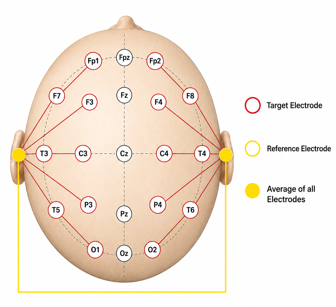
The image was adapted from López et al. (2016). In most cases, the midline electrodes are also included in these calculations.
Recording
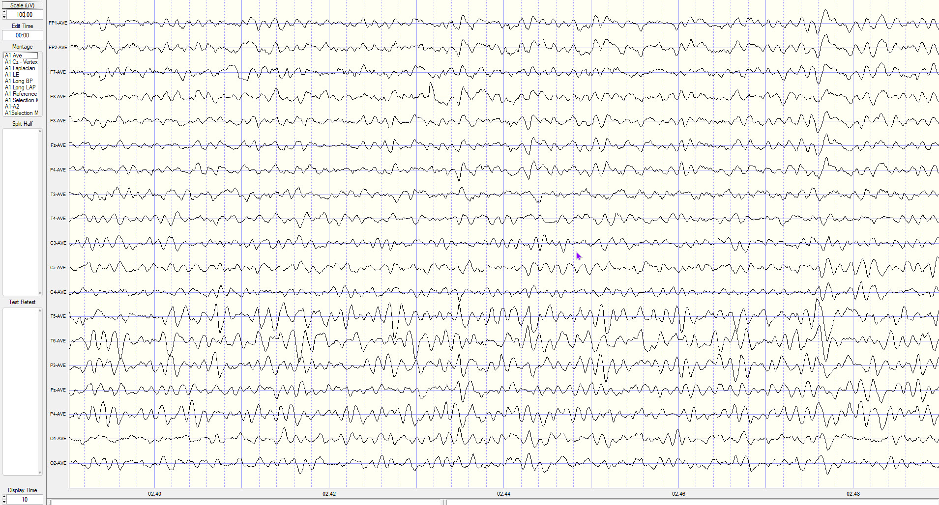
Average Reference Montage (Ave Ref) — This view shows clear anterior–posterior differences in location, along with reduced power compared with the longitudinal bipolar montage owing to the montage's averaging effect.
Strengths
The main advantage of this montage is that it replaces a single physical reference site—which is never electrically silent—with a computed, spatially distributed one, providing approximate spatial neutrality. It is not truly "reference-free"; the average itself is a reference, and its neutrality depends on the assumptions described above. It is particularly useful for visualizing diffuse, low-amplitude cerebral activity, including generalized spike-wave discharges, slow-wave abnormalities, and subtle background fluctuations. Because every electrode is displayed against the same computed reference, spatial comparisons across channels are more direct, making this montage highly valuable in qEEG and source localization studies (Fisch, 1999).
Limitations
However, this montage is highly susceptible to contamination by a single noisy electrode. If one electrode produces a high-amplitude artifact (from muscle activity or movement, for example), it shifts the computed average and distorts every channel in the display. The zero-sum assumption is also only approximately valid, and it degrades further when electrodes are unevenly distributed or confined to the upper head surface, as they are in the 10-20 array, or when cortical activity is spatially unbalanced (Nunez & Srinivasan, 2006).
Cz Reference Montage
The Cz reference montage is a referential (monopolar) configuration in which every scalp electrode is referenced to a single, fixed electrode at the vertex (Cz). This straightforward setup provides consistent spatial orientation for each channel and is used in event-related potential (ERP) research and in some pediatric recordings, where ease of interpretation and temporal clarity are priorities. Note that clinical sleep staging follows a different convention: the American Academy of Sleep Medicine specifies mastoid-referenced derivations (F4-M1, C4-M1, O2-M1), not a Cz reference.
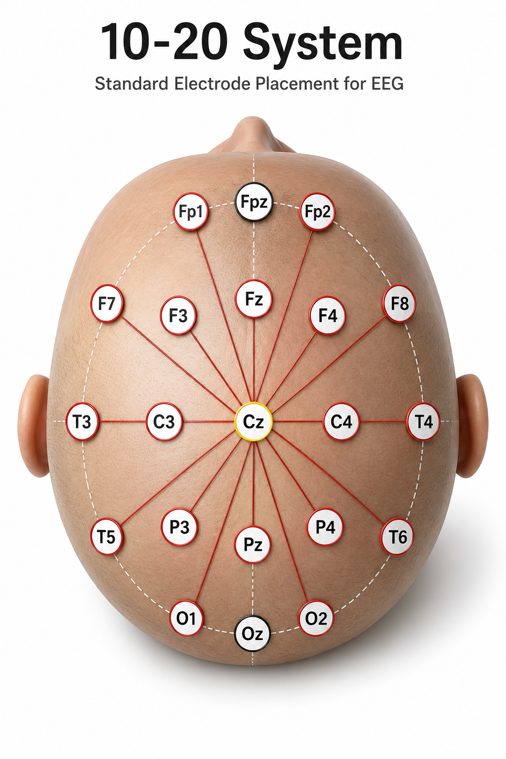
We adapted this image from López et al. (2016). In most cases, the midline electrodes are also included in these calculations.
Recording
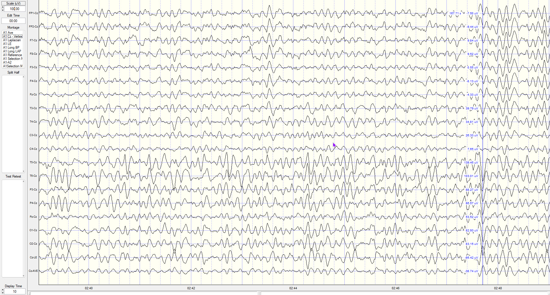
The Cz or Vertex Montage (Cz) also does not show phase reversals, since those are identified across adjacent electrode pairs. However, this montage shows larger voltage differences for electrode locations further from the Cz reference. This is particularly true for the T5 and T6 electrodes, which at the indicated point show 139.45 µV and 103.01 µV respectively. This illustrates differential amplification: what survives is whatever differs between the two inputs, while activity shared by both is rejected. The further an electrode is from a fixed reference like Cz, the less activity it shares with that reference and the more is retained.
Strengths
Because Cz is equidistant from both hemispheres, lateralized discharges produce strong voltage differences and clear waveforms. The fixed reference also facilitates temporal alignment of discharges, which is useful for assessing spike timing, propagation patterns, and hemispheric synchrony.
Limitations
Cz is a problematic reference for activity that originates near the vertex itself, such as discharges from the supplementary motor area, parasagittal cortex, or midline regions. When the reference is physically close to the source, the recorded potential difference may be minimal or absent, leading to false negatives. This limitation is particularly relevant when interpreting generalized or midline spike-wave complexes or high-frequency sleep spindles that originate near central sites (Niedermeyer & da Silva, 2005).
Linked Ears Reference (A1-A2 reference or LE) Montage
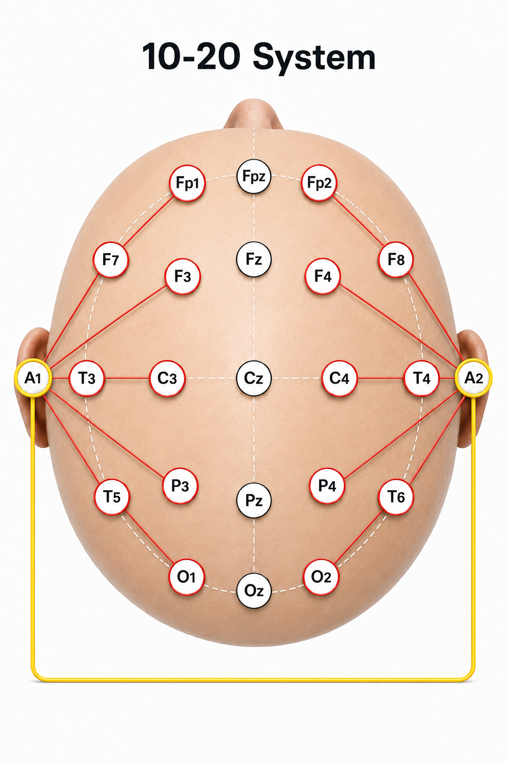
The linked ears reference montage references all scalp electrodes to the average of the left (A1) and right (A2) earlobe electrodes. These electrodes are presumed to be relatively inactive compared with cerebral sources, providing a convenient common baseline for assessing cortical activity. This montage has been widely used in routine clinical EEG and in quantitative EEG because of its simplicity and because most normative databases were collected with it (Niedermeyer & da Silva, 2005).
Two cautions apply. Physically shorting A1 and A2 together with a jumper lowers the impedance across the head and can shunt and distort genuine interhemispheric asymmetries; for this reason most modern systems compute the linked-ears reference mathematically as the average of the two separately recorded ear channels rather than wiring them together. And, as the recordings below illustrate, the ears are not silent, so the linked-ears reference introduces reference contamination into every channel.
Recording
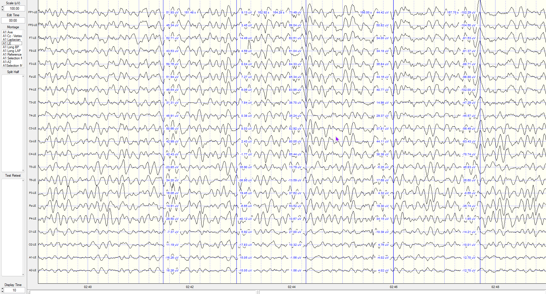
Linked Ears Montage – Scale 100uV, Display time 10 seconds. This montage shows significant synchronous activity due to reference contamination.
Notice the two reference tracings across the bottom of the image contain what appear to be EEG waveforms. These tracings represent the reference electrodes A1 and A2 (auricular left and right respectively) compared to the linked ears reference, which is the average of the two reference electrode channels: ChannelLE = channelraw − [(A1 + A2) ÷ 2].
Because the reference value is subtracted from every channel, any cerebral activity present in the ears is injected into all of them with inverted polarity. Where the scalp site carries little of that activity (mostly frontal), it appears added; where the scalp site already carries it (mostly parietal and occipital), it is partly cancelled. This is a consequence of differential subtraction, not of common-mode rejection working as intended.
Note in the image above that the prefrontal or frontal pole Fp1 and Fp2 electrodes have the highest amplitude and that O1 and O2 have the lowest. In the Average Reference Montage image below the posterior temporal, parietal and occipital sensors show the highest voltage while frontal, central and temporal show lower values.
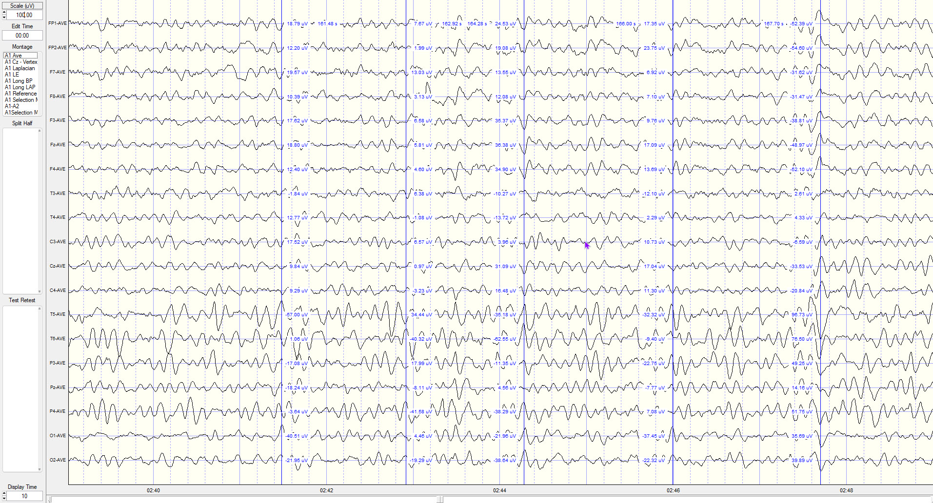
In this Average Reference Montage image, the posterior temporal, parietal and occipital sensors show the highest voltage while frontal, central and temporal show lower values.
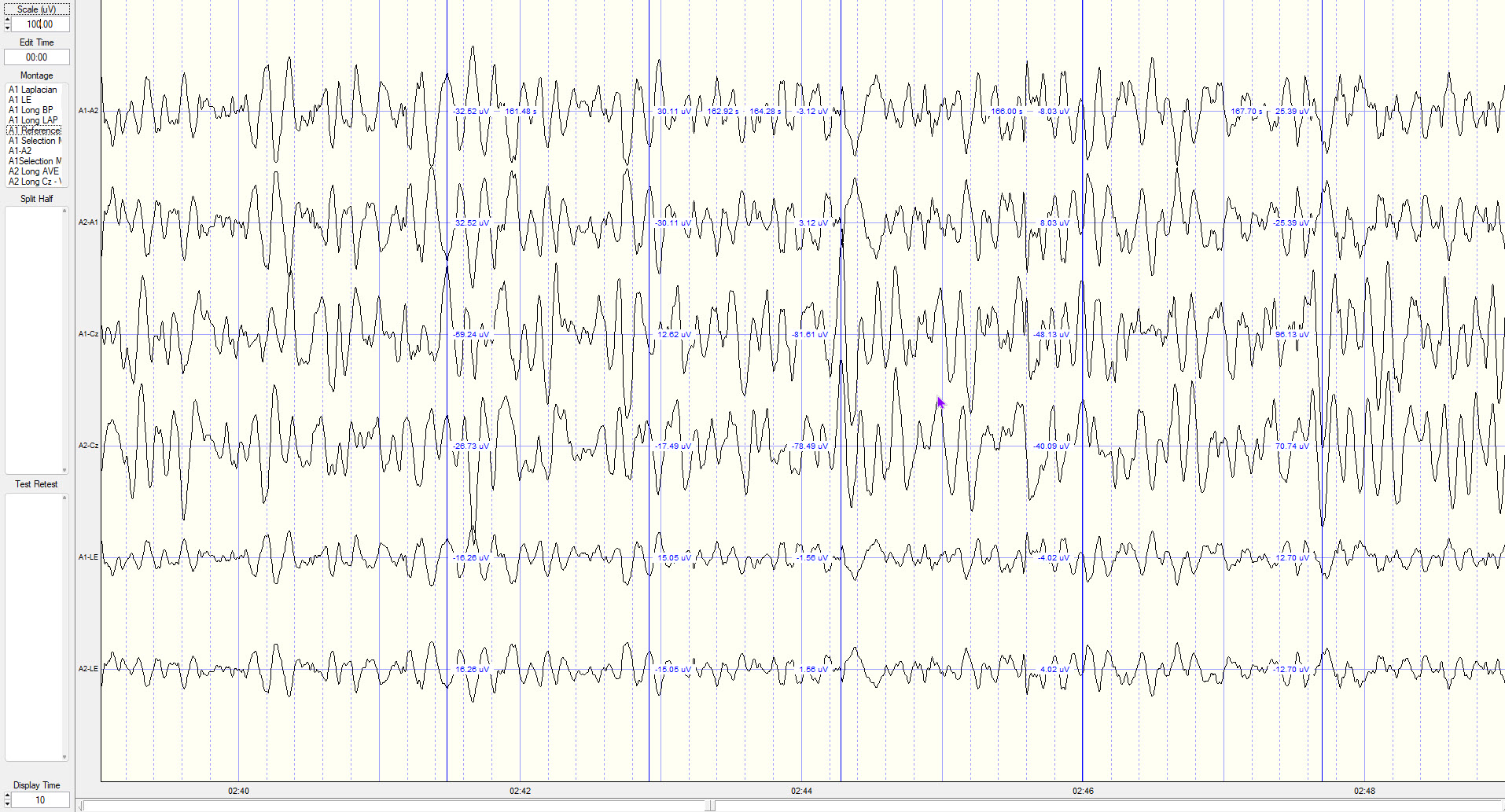
This is a created montage showing the ear references in differing combinations, e.g., A1-A2, A2-A1, A1-Cz, A2-Cz and finally A1-LE and A2-LE.
Note that the first two tracings have reverse polarity – the waves are waving in the opposite direction – as would be expected with that comparison. The initial blue vertical voltage indicator shows the first A1-A2 tracing with the right side A2 electrode as more electrically negative and the second voltage indicator for that same tracing shows the left side A1 electrode as more electrically negative. This shows the "alternating current" nature of the EEG recording.
The second two tracings show waveforms with some phase similarity but it appears from visual inspection that the voltage is somewhat higher on the left (A1-Cz).
The final two tracings show A1 and A2 compared to the average of the two electrode values and clearly show they are exactly opposite in phase as would be expected from the formula.
However, the bottom line is that the reference channels and the derivative LE linked ears channel contain EEG waveforms that will be propagated into every channel as noted above.
Strengths
The primary strength of the linked ears montage is its relative ease of interpretation and its ability to provide clear visualization of regional asymmetries. Because all electrodes share a common reference point, focal abnormalities such as interictal epileptiform discharges are often well-demarcated, especially when lateralized. Placing the reference off the scalp proper also avoids projecting vertex-region cerebral activity into every channel, as a Cz reference does, and it is the reference used by most qEEG normative databases (Nuwer, 1997).
Limitations
However, the assumption that the earlobes are electrically inactive is not valid. The ears routinely pick up cerebral activity—especially temporal and posterior activity, and particularly during high-amplitude discharges—which is then injected into the reference and, through the differential amplifier, into every channel (Gloor, 1985). Because the earlobes sit close to the temporalis and posterior neck muscles, they are also a common entry point for EMG contamination. Asymmetry in earlobe impedance or local artifact can produce lateralized distortions that mimic or obscure true cerebral asymmetries, and the reference may underrepresent midline or deep sources.
Laplacian Montage
The Laplacian montage enhances the localization of cortical activity by referencing each electrode to a weighted average of its surrounding electrodes. This approach approximates the second spatial derivative of the potential field, emphasizing signals originating directly beneath each electrode while attenuating distant or volume-conducted signals (Nunez & Srinivasan, 2006). Think of it as a spatial "sharpening filter" for EEG data.
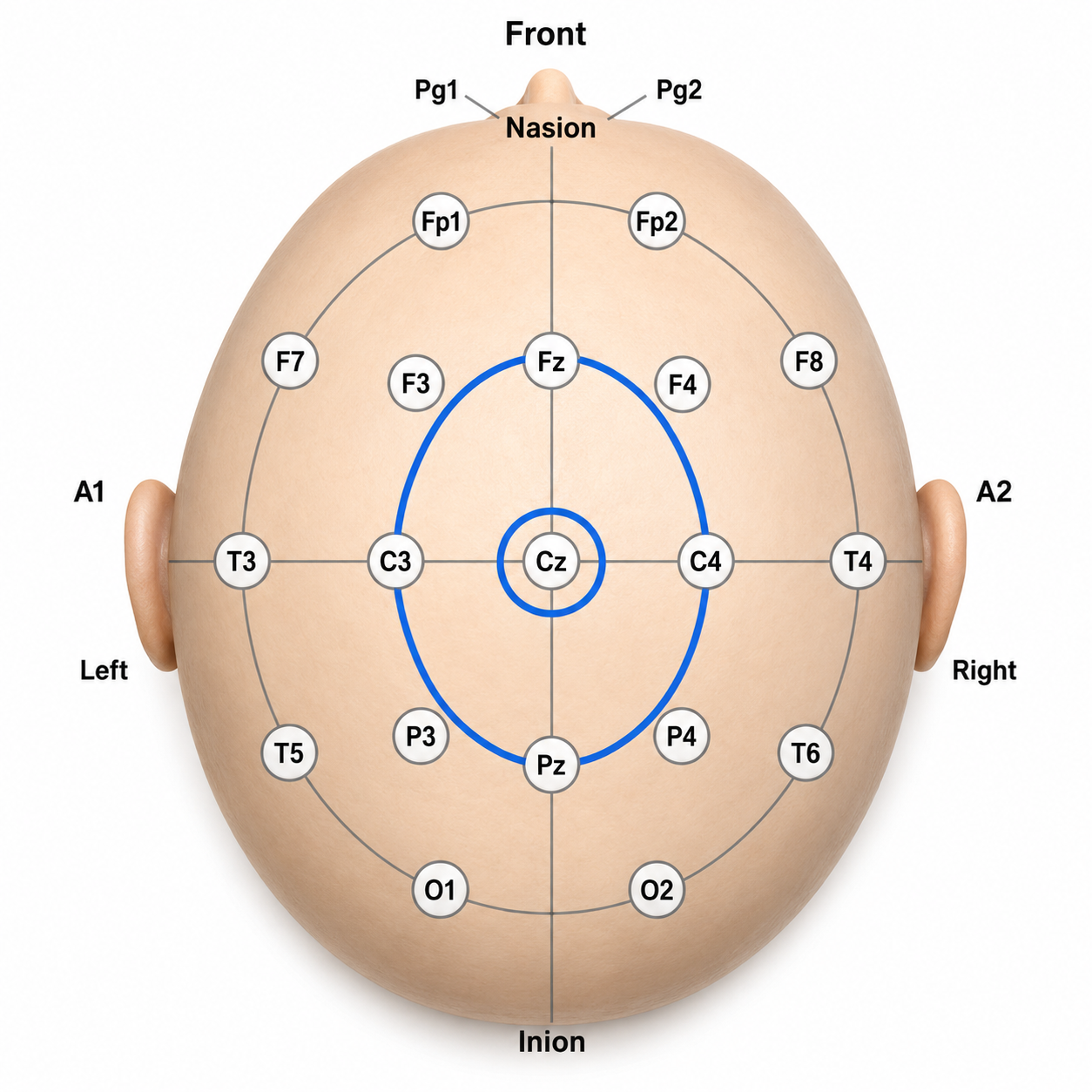
In a Laplacian montage, the signal at a target electrode is compared with the activity of surrounding electrodes to estimate local scalp potential and reduce broad, volume-conducted activity. The small blue circle around Cz identifies it as the central target electrode. The larger blue oval identifies the neighboring electrodes used as the surrounding reference field, chiefly Fz, C3, C4, and Pz. Cz is emphasized, while more diffuse activity shared across nearby electrodes is subtracted out. This makes focal central activity easier to see and helps improve spatial localization compared with a conventional referential montage.
Recording
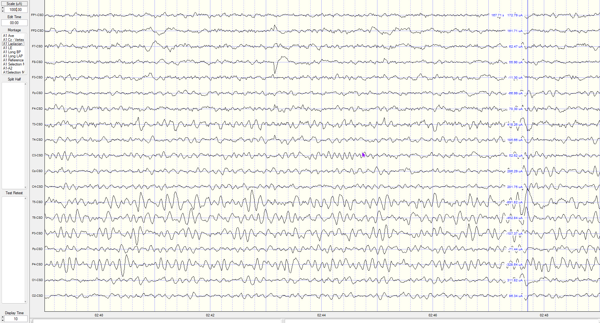
The Laplacian Montage (LAP) displays an estimate of current source density (CSD) rather than voltage. Strictly speaking, the surface Laplacian has units of potential per unit area (commonly µV/cm²); some software labels the axis in current units such as µA, which should be read as a software convention rather than a literal current measurement. This montage, too, does not show phase reversals in the conventional sense.
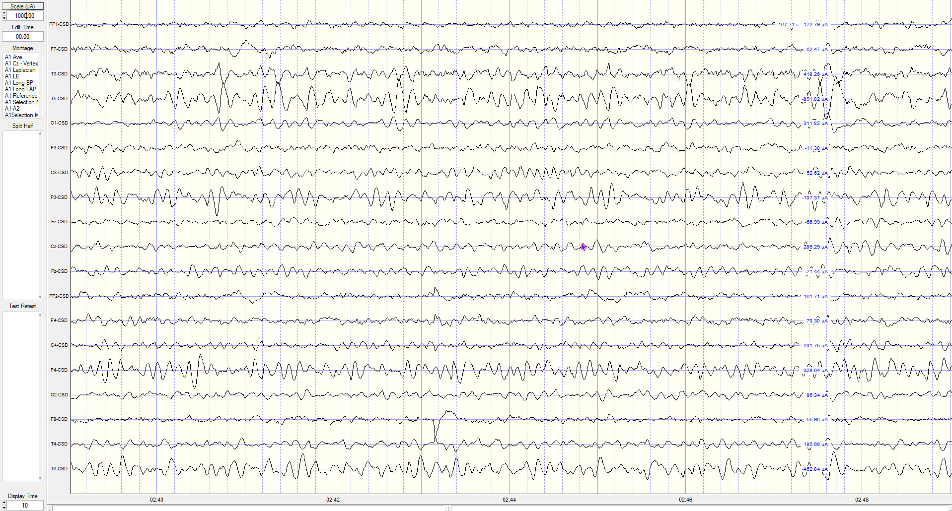
However, in this non-traditional view that applies an anterior–posterior electrode-chain approach similar to the Long BP montage, comparable phase-reversal information appears to be present—between T3-CSD and T5-CSD, and between T5-CSD and O1-CSD.
Strengths
The Laplacian montage offers significant advantages for localizing focal cortical activity with high spatial precision. Unlike referential montages that rely on ear or mastoid electrodes, this configuration excludes distant references, minimizing the risk of artifact from electrically active or asymmetrically placed reference sites. It is particularly effective for detecting focal epileptiform discharges, localized slowing, and sensorimotor rhythms, especially when applied in high-density EEG systems (McFarland et al., 1997). While not typically used as a primary montage, it serves as a valuable supplementary tool for refining diagnostic accuracy in complex cases.
Limitations
The Laplacian montage's accuracy depends on high-density, evenly spaced electrode arrays, making it less reliable in standard low-density systems like the 10-20 configuration. A key concern is the edge effect: electrodes at the scalp periphery (such as Fp1, Fp2, F7, F8, O1, and O2) lack surrounding electrodes on all sides, reducing the precision of spatial averaging in these regions. Additionally, the spatial filtering inherent to this method attenuates slow or widespread activity, limiting its sensitivity to generalized abnormalities such as diffuse slowing or generalized spike-wave discharges (Gordon & Rzempoluck, 2004; Srinivasan et al., 1996).
Montage Selection Strategy
When viewing the EEG, your goal is to identify areas that deviate from typical patterns, correlate those differences with client symptoms, and design training protocols to address them. Each montage reveals different aspects of the same data. The longitudinal bipolar and transverse montages are most effective at demonstrating focal abnormalities, with clear localization, polarity, and sharp morphology, making them essential for identifying epileptiform discharges and mapping their spatial distribution.
The average reference montage, while less sensitive to focal events, contributes significantly to assessing hemispheric symmetry and background rhythm integrity, particularly in diffuse or generalized processes. The Cz reference montage provides a reliable lateralized perspective for differentiating left versus right hemispheric activity, though it lacks optimal resolution for midline sources. The linked ears reference offers consistency in visualizing lateralized abnormalities but can introduce asymmetry and contamination, especially with poor electrode impedance.
The Laplacian montage offers superior spatial resolution for identifying focal cortical sources by emphasizing activity local to each electrode and suppressing distant or volume-conducted activity. Understanding the comparative strengths and limitations of each montage enables more nuanced and precise interpretation of EEG findings, enhancing diagnostic accuracy and supporting informed clinical decision-making.
Re-Montaging
In clinical electroencephalography, the montage used to display data fundamentally shapes how brain activity is visualized and interpreted. An essential feature of modern digital EEG is that clinicians are not limited to a single display: they can apply different montages to the same epoch of data. This process, known as re-montaging, allows for a more complete understanding of the recorded activity.
Modern EEG visualization software also allows clinicians to create custom montages that highlight selected electrodes, use alternative electrode arrangements, or follow non-standard sequences. For example, grouping all frontal electrodes at the top of the page makes eye artifact easier to identify, while grouping temporal electrodes together facilitates EMG artifact detection.
The narrated video below © John S. Anderson displays the same 21-channel recording viewed using different montages with a 60-Hz notch filter on and off.
Re-montaging enables clinicians to re-express the same underlying electrical signals in different spatial contexts. A spike that shows a clear phase reversal in a longitudinal bipolar montage may appear attenuated in an average reference montage. Conversely, a sharply contoured waveform seen in a bipolar montage can be cross-checked in a referential montage to determine whether it reflects true cortical activity or a muscle artifact. This comparative approach is essential for avoiding misinterpretation, particularly when benign variants or technical artifacts could be mistaken for pathologic activity.
Re-montaging also improves localization. By switching between longitudinal and transverse configurations, you can more precisely triangulate the source of epileptiform discharges and determine whether a waveform is confined to one hemisphere or crosses the midline. In suspected encephalopathy, re-montaging into an average reference montage may better demonstrate diffuse slowing or triphasic waves. Following the average reference, the Laplacian montage can help zero in on areas of interest, while the linked ears montage should be consulted to identify likely reference contamination affecting downstream evaluations such as topographic z-score maps, coherence, and network analyses.
Digital EEG systems have made re-montaging straightforward and immediate. The American Clinical Neurophysiology Society recommends the use of both bipolar and referential montages and encourages at least 16 recording channels with the full complement of 10-20 system electrodes. When you identify an EEG feature, such as slowed alpha, elevated frontal theta, excess fast activity, or an atypical alpha response, in one montage, always verify and validate that finding using additional montages.
Use Consistent Settings
One important consideration for viewing the EEG is to use consistent display settings. In clinical EEG, the conventional standards are a sensitivity of 7 μV/mm and a "chart speed" of 30 mm per second; neurofeedback software often expresses the vertical axis instead as a fixed scale marker, commonly 50 or 100 μV. In the era of paper recording, tracings were drawn by pens on moving chart paper at 30 mm/s for routine adult and pediatric recordings, with slower speeds such as 15 mm/s used for neonatal and sleep studies. Modern digital systems replicate this format so that waveforms appear consistently the same each time they are viewed and can be compared to reference sources.
Most modern EEG software expresses display time in seconds rather than chart speed equivalents. At 30 mm/s, a standard page corresponds to 10 seconds of data, which is the setting to select in programs such as NeuroGuide; note that in some display modes the vertical scale adjusts automatically to the highest voltage in the recording, which will change the apparent amplitude from page to page unless it is fixed.
Best Practices from the American Clinical Neurophysiology Society Guideline 3 (2016)
The Committee reaffirms the statements pertaining to montages set forth previously in the Guidelines of the American Clinical Neurophysiology Society (ACNS) and that are paraphrased as follows:
(a) that no less than 16 channels of simultaneous recording be used, and that a larger number of channels be encouraged,
(b) that the full 21 electrode placements of the 10-20 system be used,
(c) that both bipolar and referential montages be used for clinical interpretation,
(d) that the electrode derivations of each channel be clearly identified at the beginning of each montage,
(e) that the pattern of electrode connections be made as simple as possible, and that montages should be easily comprehended,
(f) that the electrode pairs (bipolar) preferentially should run in straight (unbroken) lines and the interelectrode distances kept equal,
(g) that tracings from the more anterior electrodes be placed above those from the more posterior electrodes on the recording page, and,
(h) that it is very desirable to have some of the montages comparable for all EEG laboratories.
2.2 The Committee recommends a "left above right" order of derivations, i.e., on the recording page, left-sided leads should be placed above right-sided leads for either alternating pairs of derivations or blocks of derivations. This recommendation coincides with the prevailing practice of most EEG laboratories, at least in North America and in many other areas.
Check Your Understanding
- Why does a single noisy channel compromise every trace in an average reference montage?
- What is the edge effect, and which montages does it affect?
- Why can the Cz reference montage underestimate vertex sharp waves?
- Which montage would you select to localize an epileptiform focus, and which to characterize a distributed resting rhythm? Justify each choice.
- Summarize the ACNS Guideline 3 recommendations for channel count, electrode placements, and page layout.
Cutting-Edge Topics in qEEG Research
Montage as a Confound in Normative Comparison
Normative databases were built with a specific reference, and comparing a client's record to a database built on a different one introduces error that no z-score will flag. Thatcher (2010) documented how tightly validity is bound to referencing choices, which is why linked ears persists long after its contamination problems became well known. The practical rule is unglamorous but important: match the montage the database was built with, and change montages for visual review rather than for statistical comparison.
Surface Laplacian and Current Source Density Move Toward Routine Use
Kayser and Tenke (2015) argued that the surface Laplacian should be a default step rather than a specialist technique, since it removes the reference problem entirely by expressing activity as radial current flow rather than as voltage relative to some other site. The obstacle has always been electrode density and the edge effect at peripheral sites. As 64-channel and higher arrays become affordable in clinical settings, expect CSD-based displays to move from research papers into ordinary reports.
How Many Channels Are Enough?
Lau and colleagues (2012) asked how many electrodes are really needed for EEG-based mobile brain imaging and found that channel count interacts with the question being asked rather than answering it outright. That framing is useful clinically: a single-channel SMR protocol at Cz does not need 19 channels, but a coherence or phase question cannot be answered without them. The cost of full arrays has fallen far enough that the honest question is now what you intend to measure rather than what you can afford.
Does Artifact Correction Distort Connectivity?
Montage choice and artifact correction interact in ways the field is still working out. Independent component analysis is applied to data in one reference and then re-referenced for display, and there is evidence that this sequence distorts phase relationships even in clean segments. For coherence and phase metrics, which are precisely the measures that justify multi-channel recording, this is not a minor methodological footnote. Documenting your reference and your correction pipeline is becoming part of what a defensible report contains.
Assignment
Now that you have completed this module, explain which montages you use in your practice and their strengths and limitations. For at least one client presentation you see regularly, describe the sequence of montages you would review and what each one would tell you that the others would not.
Glossary
50/60 Hz artifact: external artifacts transmitted by nearby electrical sources such as power lines.
active electrode: an electrode positioned at a measurement site whose potential contributes to the recorded differential signal; it is distinct from the reference and ground electrodes.
amplitude: the magnitude of a signal's excursion from a specified reference level, reported using a stated convention such as peak, peak-to-peak, or RMS.
average-reference montage: an EEG montage in which each channel represents an electrode's potential relative to the instantaneous average of a specified set of electrodes.
bipolar montage: an EEG montage composed of bipolar derivations, often arranged in longitudinal or transverse chains to emphasize spatial voltage gradients.
cardiac artifact: ECG or pulse-related activity that appears in an EEG channel through electrical or mechanical coupling. It should not be interpreted as cerebral activity or as a cardiac diagnosis.
channel: one differential amplifier input, formed by a pair of electrodes whose voltage difference is recorded. A single ground electrode is shared across all channels rather than belonging to any one of them.
circular (circumferential) bipolar montage: a bipolar configuration in which adjacent electrodes are chained around the perimeter of the head.
coherence (EEG): a frequency-specific measure equal to the squared magnitude of the cross-spectrum divided by the product of the two autospectra, ranging from 0 to 1.
common average montage: a reference montage in which each electrode's potential is compared with the mean of all recording electrodes, sometimes computed from a selected subset that excludes noisy or edge channels.
common-mode rejection: a differential amplifier's suppression of voltage shared by both inputs while amplifying the voltage difference between them.
common-mode rejection ratio (CMRR): the ratio of differential gain to common-mode gain, commonly expressed in decibels, indicating rejection of signals shared by both inputs.
comodulation: covariation over time in the amplitude or power of a specified frequency band between recording sites, calculated with a stated method.
current source density (CSD): a technique used in source derivation montages that estimates the local net current flow into or out of the scalp at a given electrode site.
Cz: the central vertex electrode located at the intersection of the midline sagittal and coronal planes on the scalp.
Cz reference montage: a referential (monopolar) configuration in which every scalp electrode is referenced to a single fixed electrode at the vertex of the scalp, providing consistent spatial orientation for each channel.
derivation: the voltage difference or computed signal produced from a specified pair or combination of recording electrodes.
differential amplifier: an amplifier that outputs a gain-scaled difference between two input voltages while suppressing voltage common to both.
edge effect: the loss of accuracy at peripheral electrodes in Laplacian and source derivation montages, where too few neighboring electrodes are available for the spatial average.
electro-ocular artifact: contamination of EEG recordings by potentials generated by eye blinks, eye flutter, and eye movements.
EMG artifact (ECG): false or obscured ECG events caused by skeletal-muscle electrical activity, potentially producing spurious or missed beat detections.
frequency: the number of complete cycles of a periodic phenomenon per unit time, expressed in hertz for cycles per second.
ground electrode: an electrode connected to the recording system's common or driven-ground circuit to reduce common-mode interference; it is distinct from the reference electrode.
hertz (Hz): the SI unit of frequency equal to one cycle per second.
international 10–10 system: an extension of the international 10–20 electrode-placement system that adds scalp locations at 10% intervals for greater spatial sampling.
international 10–20 system: a standardized method for locating EEG electrodes at intervals of 10% or 20% of measured head distances; the original array includes 19 scalp and two auricular sites, with ground specified separately.
Laplacian montage: a spatially filtered EEG montage comparing each electrode with a weighted average of nearby electrodes to emphasize local radial activity.
linked ears montage: an EEG montage that uses the average of both earlobe or mastoid electrodes as the reference for all other electrodes.
longitudinal bipolar montage (double banana): an EEG recording configuration involving the anterior-to-posterior chaining of adjacent electrodes in two lines on each side (Fp1 to O1 and Fp2 to O2) and connecting the midline electrodes (Fz to Pz).
microvolt (µV): a unit of electric potential equal to 10⁻⁶ volt.
monopolar recording: a historical term for referential recording in which an active electrode is compared with a relatively inactive reference; a separate ground electrode is also used.
montage: the specified arrangement of electrode derivations or channel pairings used to display a physiological recording.
mu rhythm: an 8 to <13 Hz arch-shaped or wicket-like EEG rhythm over central sensorimotor regions that attenuates with movement or somatosensory activation.
phase: the position of a periodic signal within its cycle, usually expressed in degrees or radians relative to a reference.
phase reversal: the polarity inversion of a waveform between adjacent derivations in a bipolar chain, which localizes the source to the shared electrode.
posterior dominant rhythm (PDR): the dominant occipital rhythm during relaxed wakefulness with eyes closed, usually in the alpha range in healthy adults and attenuated by eye opening.
quantitative EEG (qEEG): the numerical analysis of digitized EEG features, such as spectral power, asymmetry, and connectivity, sometimes compared with normative databases; no universal minimum channel count defines it.
reference contamination: the erroneous inclusion of signals from the reference electrode into the EEG trace of the active electrode.
reference electrode: an electrode whose potential is used as the comparison for an active recording electrode; it is distinct from the ground electrode.
referential montage: an EEG montage in which multiple active electrodes are each compared with the same reference electrode or reference combination.
sensorimotor rhythm (SMR): a 12 to 15 Hz rhythm recorded over sensorimotor cortex, enhanced during physical stillness and attenuated by movement; it is defined topographically and behaviorally, so its range overlaps the mu and beta bands.
sequential (bipolar) montage: a recording method that presents a sequence of comparisons between pairs of active electrodes attached to sites on the scalp, with no shared reference.
source derivation montage: a montage using mathematical algorithms, such as CSD, to estimate the underlying cortical generators of scalp-recorded EEG signals.
transverse bipolar montage: a bipolar configuration in which adjacent electrodes are chained from left to right across the head rather than front to back.
vertex and Cz: the vertex is the highest point of the skull; Cz is the midline EEG position at the intersection of nasion-inion and left-right preauricular measurements.
vertex sharp wave: a midline EEG waveform typically seen during drowsiness, originating near the Cz electrode.
Test Yourself on ClassMarker
Click the button below to take a 10-question exam over this entire unit. There is no password.
Review Flash Cards on Quizlet
Click the button below to review our chapter flash cards.
References
Acharya, J. N., Hani, A. J., Thirumala, P. D., & Tsuchida, T. N. (2016). American Clinical Neurophysiology Society Guideline 3: A proposal for standard montages to be used in clinical EEG. Journal of Clinical Neurophysiology, 33(4), 312–316. https://doi.org/10.1097/WNP.0000000000000317
Carvalhaes, C., & de Barros, J. A. (2015). The surface Laplacian technique in EEG: Theory and methods. International Journal of Psychophysiology, 97(3), 174–188. https://doi.org/10.1016/j.ijpsycho.2015.04.023
Demos, J. N. (2019). Getting started with EEG neurofeedback (2nd ed.). W. W. Norton & Company.
Gasser, T., Bächer, P., & Steinberg, H. (1985). Test-retest reliability of spectral parameters of the EEG. Electroencephalography and Clinical Neurophysiology, 60(4), 312–319. https://doi.org/10.1016/0013-4694(85)91066-0
Gordon, E., & Rzempoluck, E. (2004). Laplacian methods and drug effects. Clinical EEG and Neuroscience, 35(2), 76–82. https://doi.org/10.1177/155005940403500207
Huigen, E., Peper, A., & Grimbergen, C. A. (2002). Investigation into the origin of the noise of surface electrodes. Medical and Biological Engineering and Computing, 40, 332–338. https://doi.org/10.1007/BF02345445
Johnstone, J., Gunkelman, J., & Lunt, J. (2005). Clinical database development: Characterization of EEG database. Journal of Neurotherapy, 9(3), 27–44. https://doi.org/10.1300/J184v09n03_04
Kayser, J., & Tenke, C. E. (2006). Principal components analysis of Laplacian waveforms as a generic method for identifying ERP generator patterns. Clinical Neurophysiology, 117(2), 348–368. https://doi.org/10.1016/j.clinph.2005.08.034
Kayser, J., & Tenke, C. E. (2015). On the benefits of using surface Laplacian (current source density) methodology in electrophysiology. International Journal of Psychophysiology, 97(3), 171–173. https://doi.org/10.1016/j.ijpsycho.2015.06.001
Lau, T. M., Gwin, J. T., & Ferris, D. P. (2012). How many electrodes are really needed for EEG-based mobile brain imaging? Journal of Behavioral and Brain Science, 2(3), 387–393. https://doi.org/10.4236/jbbs.2012.23044
Lüders, H. O., Acharya, J. N., & Baumgartner, C. (2000). Semiology of epilepsy. Handbook of Clinical Neurology, 97, 21–51. https://doi.org/10.1016/S0072-9752(10)97003-2
MettingVanRijn, A. C., Peper, A., & Grimbergen, C. A. (1990). High-quality recording of bioelectric events: Part 1. Interference reduction, theory and practice. Medical and Biological Engineering and Computing, 28, 389–397. https://doi.org/10.1007/BF02441961
Niedermeyer, E., & da Silva, F. L. (2005). Electroencephalography: Basic principles, clinical applications, and related fields (5th ed.). Lippincott Williams & Wilkins.
Nunez, P. L., & Srinivasan, R. (2006). Electric fields of the brain: The neurophysics of EEG (2nd ed.). Oxford University Press.
Nuwer, M. R. (1997). Assessment of digital EEG, quantitative EEG, and EEG brain mapping: Report of the American Academy of Neurology and the American Clinical Neurophysiology Society. Neurology, 49(1), 277–292. https://doi.org/10.1212/WNL.49.1.277
Perrin, F., Pernier, J., Bertrand, O., & Echallier, J. F. (1989). Spherical splines for scalp potential and current density mapping. Electroencephalography and Clinical Neurophysiology, 72(2), 184–187. https://doi.org/10.1016/0013-4694(89)90180-6
Picton, T. W., Bentin, S., Berg, P., Donchin, E., Hillyard, S. A., Johnson, R., Miller, G. A., Ritter, W., Ruchkin, D. S., Rugg, M. D., & Taylor, M. J. (2000). Guidelines for using human event-related potentials to study cognition: Recording standards and publication criteria. Psychophysiology, 37(2), 127–152. https://doi.org/10.1111/1469-8986.3720127
Sanei, S., & Chambers, J. A. (2007). EEG signal processing. Wiley-Interscience. https://doi.org/10.1002/0470035930
Srinivasan, R., Nunez, P. L., & Silberstein, R. B. (1996). Spatial filtering and neocortical dynamics: Estimates of EEG coherence. IEEE Transactions on Biomedical Engineering, 43(7), 712–720. https://doi.org/10.1109/10.502603
Stern, R. M., Ray, W. J., & Quigley, K. S. (2001). Psychophysiological recording (2nd ed.). Oxford University Press.
Tatum, W. O. (2014). Handbook of EEG interpretation (2nd ed.). Demos Medical Publishing.
Tenke, C. E., & Kayser, J. (2012). Generator localization by current source density: Implications of volume conduction and field closure at intracranial and scalp resolutions. Clinical Neurophysiology, 123(12), 2328–2345. https://doi.org/10.1016/j.clinph.2012.06.005
Thatcher, R. W. (2010). Validity and reliability of quantitative EEG. Journal of Neurotherapy, 14(2), 122–152. https://doi.org/10.1080/10874201003773500
Thomas, C. (2007). What is a montage? EEG instrumentation. American Society of Electroneurodiagnostic Technologists.
Thompson, M., & Thompson, L. (2015). The neurofeedback book: An introduction to basic concepts in applied psychophysiology (2nd ed.). Association for Applied Psychophysiology and Biofeedback.
Return to Top