
Current Source Density Maps, Metrics, and Graphic Methods
What You Will Learn in This Chapter
Imagine trying to locate a whispering conversation by listening through a thick wall. You hear something, but the wall smears the sound so badly that you cannot tell which room it came from. That is roughly what raw scalp EEG does to cortical activity. Skull, cerebrospinal fluid, and scalp blur every signal by volume conduction, so a voltage recorded at Cz may have been generated centimeters away.
Current source density analysis is the sharpening tool. By taking spatial derivatives of the voltage field, it estimates where current enters the extracellular space (sinks) and where it leaves (sources), and it does so without depending on the reference electrode you happened to choose. In this unit you will learn how CSD maps are generated, the three metrics that quantify them, and the graphic methods used to display them, including color maps, contour plots, 3D surface plots, and time-series plots.
You will also meet the inverse-solution family that dominates clinical qEEG practice: LORETA, sLORETA, and eLORETA, along with the related VARETA and swLORETA solutions, and the voxels and Talairach coordinates that give their output an anatomical address. You will see how source-space normative databases turn those estimates into z-scores that a clinician can act on. Finally, you will compare those inverse solutions with surface Laplacian analysis, which reaches a similar goal by an entirely different route and makes far fewer assumptions along the way.
IQCB Blueprint Coverage: This unit addresses Current Source Density Maps, Metrics, and Graphic Methods (V.G) within qEEG (V).
Learning Objectives
After completing this section, you will be able to:
Define current source density mapping and explain how it differs from raw voltage recording.
Describe the preprocessing and derivative steps used to generate a CSD map from EEG or local field potential data.
Distinguish source strength, source distribution, and source dynamics, and state the units and clinical question each addresses.
Compare color maps, contour plots, 3D surface plots, and time-series plots, and select the display that best answers a given question.
Explain how LORETA, sLORETA, and eLORETA differ in resolution, units, and claimed localization error.
Describe how VARETA and swLORETA extend the LORETA approach, and state what each adds and what each still cannot deliver.
Describe voxels and Talairach coordinates and explain why stereotaxic coordinates transfer across imaging modalities.
Explain how source-space normative databases convert current density estimates into z-scores, and summarize the evidence for their reliability and validity.
Contrast surface Laplacian analysis with the LORETA family of inverse solutions with respect to reference dependence and modeling assumptions.
Summarize the basic and clinical research applications of CSD analysis.
Listen to the Full-Length Lecture
What Current Source Density Analysis Measures
Current source density (CSD) mapping is a method used to determine the locations and magnitudes of current sources and sinks within the brain. It works by analyzing the spatial distribution of voltage gradients recorded by electrodes, typically in the form of electroencephalography (EEG) or local field potentials (LFPs).
By applying mathematical transformations to those data, you can create detailed maps that reveal the underlying neural activity with high spatial resolution (Nicholson & Freeman, 1975). The technique is powerful precisely because it does not ask you to trust the raw voltage. It asks you to trust the shape of the voltage field, which carries information the raw numbers hide.
Current Source Density Maps
CSD maps visualize where electrical currents enter the extracellular space and where they leave it. Current entering the extracellular space marks a sink, and current leaving it marks a source. These maps are created by differentiating the voltage signals recorded at multiple spatially arranged electrodes.
The resulting data show the spatial distribution of neuronal activity far more clearly than raw voltage recordings do. The reason is volume conduction, the passive spread of current through brain, skull, and scalp tissue, which smears activity across the head and obscures the true locations of neuronal generators. CSD analysis largely eliminates that influence (Freeman & Nicholson, 1975).
How CSD Maps Are Generated
Generating a CSD map begins with housekeeping. The recorded EEG or LFP data are first preprocessed to remove noise and artifacts, because a spatial derivative amplifies high-frequency noise as readily as it amplifies signal.
Next, the voltage differences between adjacent electrodes are calculated to obtain the first spatial derivative. A second derivative is then computed to produce the CSD values, which represent the current density at each point in the electrode array. Those values are finally visualized as maps in which color gradients indicate the intensity and direction of current flow (Poghosyan & Ioannides, 2007).
Notice what this two-step derivative buys you. The first derivative tells you how steeply voltage changes across the scalp, and the second tells you where current must be entering or leaving to produce that steepness. That is why the method is sometimes described as reading the curvature of the voltage field rather than its height.
Metrics Used in CSD Analysis
CSD analysis involves several key metrics that provide quantitative insights into the characteristics of neuronal sources and sinks. Each answers a different question: how strong, where, and when.
Source Strength
Source strength quantifies the magnitude of current sources and sinks. It is typically expressed in units of current density (A/m²) and provides a measure of the intensity of neuronal activity at different locations within the brain (Tenke et al., 2015).
Source Distribution
Source distribution describes the spatial extent and distribution of current sources and sinks. You can use it to identify patterns of neural activation and to determine the localization of functional areas within the cortex (Kayser & Tenke, 2006).
Source Dynamics
Source dynamics refers to the temporal changes in current density over time. This metric is crucial for understanding the timing and sequence of neural events, which matters especially in studies of sensory processing and cognitive function (Mitzdorf, 1985).
CSD mapping estimates the locations and magnitudes of current sources and sinks by taking spatial derivatives of the voltage field recorded across an electrode array. The first derivative captures the voltage gradient between adjacent electrodes, and the second derivative yields the current density at each point. Because the method reads the shape of the field rather than its absolute height, it largely removes the blurring caused by volume conduction. Three metrics quantify the result: source strength in A/m², source distribution across the cortex, and source dynamics over time.
Check Your Understanding
- What is the difference between a current source and a current sink in CSD terminology?
- Why must EEG or LFP data be cleaned of noise and artifacts before the derivatives are computed?
- What does the second spatial derivative provide that the first one does not?
- Which CSD metric would you examine to determine whether a response peaks before or after a stimulus, and why?
- Explain in your own words how volume conduction degrades the interpretability of raw scalp voltages.
Graphic Methods for Representing CSD Data
Graphical representation of CSD data is essential for interpreting the spatial and temporal patterns of neuronal activity. Several methods are commonly used, and each trades one kind of clarity for another. Your choice of display should follow the question you are asking.
Color Maps
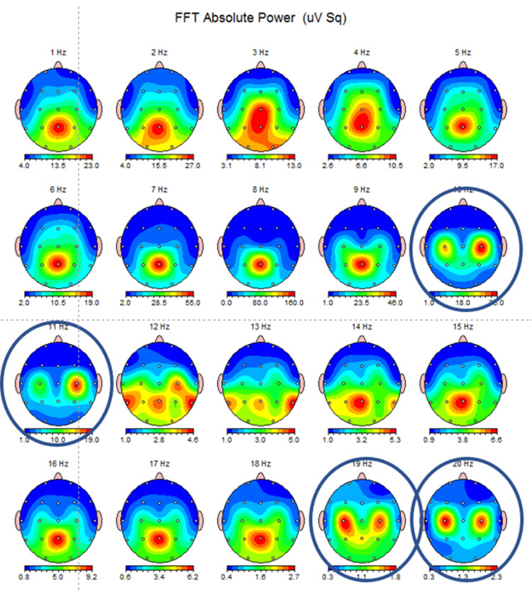
Color maps are one of the most common methods for displaying CSD data. In these maps, different colors represent different magnitudes of current density, with gradients indicating the intensity and direction of currents. Color maps provide an intuitive and easily interpretable visualization, which makes it easy to spot areas of high activity at a glance (Tenke et al., 2015).
Contour Plots
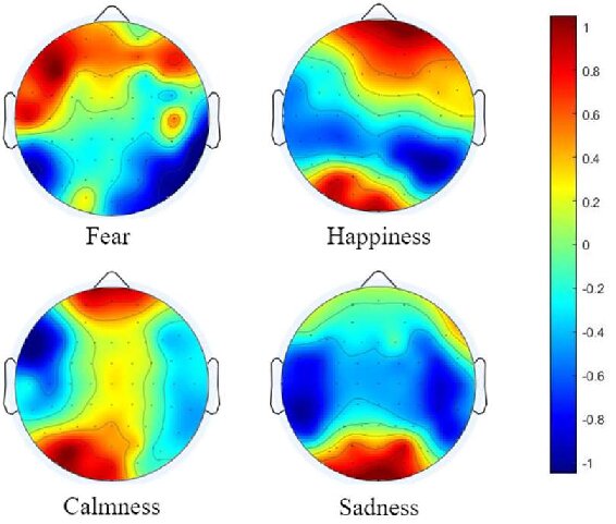
Contour plots use lines to represent areas of equal current density, much like the topographic maps used in geography. These plots are useful for identifying the precise locations of sources and sinks and for visualizing the spatial structure of neural activity (Freeman & Nicholson, 1975). Where a color map gives you an impression, a contour plot gives you a boundary.
3D Surface Plots
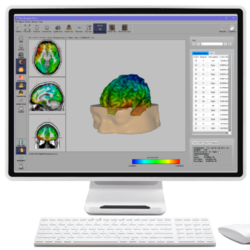
3D surface plots provide a three-dimensional representation of CSD data in which the height of the surface corresponds to the magnitude of current density. These plots offer a more detailed view of the spatial distribution of neural activity, making it easier to identify complex patterns and interactions between brain regions (Nicholson & Freeman, 1975).
Time-Series Plots
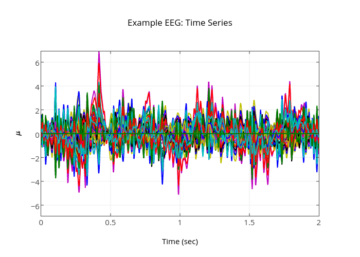
Time-series plots display the temporal evolution of CSD values at specific locations or across the entire electrode array. These plots are crucial for understanding the dynamics of neural activity and for correlating CSD data with behavioral or sensory events (Mitzdorf, 1985).
LORETA, sLORETA, and eLORETA
Source localization addresses the EEG inverse problem, the challenge of estimating which cortical generators produced a recorded pattern of scalp voltages, because many different source configurations can produce the same surface recording (Thompson & Thompson, 2015).
Low resolution electromagnetic tomography (LORETA) is Pascual-Marqui, Michel, and Lehmann's (1994) mathematical inverse solution for identifying the cortical sources of 19-electrode quantitative data acquired from the scalp. In this context, tomography refers to two-dimensional coronal, horizontal, and sagittal brain slices.
Be clear about what LORETA cannot do. LORETA's solution space is restricted to cortical gray matter, plus hippocampus in the original implementation. Structures outside that space (thalamus, amygdala, basal ganglia, brainstem, and cerebellum) contain no voxels and therefore cannot be identified as sources (Thompson & Thompson, 2015). A client report that claims a thalamic generator on the basis of a 19-channel LORETA image is claiming more than the method supports. That limit belongs to the classic LORETA and sLORETA solution spaces; later weighted variants enlarge the solution space to include selected subcortical structures, a development taken up under Weighted LORETA and Subcortical Solution Spaces below.
Voxels and Talairach Coordinates
LORETA represents cortical sites using three-dimensional voxels, which are volumetric units. Its original voxels had a 7-mm spatial resolution, measuring 7 mm by 7 mm by 7 mm, and that resolution has since improved to 5 mm by 5 mm by 5 mm. LORETA values are expressed as current density in amperes per square meter (A/m², equivalently µA/mm²).
LORETA assigns each voxel x, y, and z Talairach coordinates referencing the original Talairach atlas and subsequent atlases such as the Montreal Neurological Institute (MNI) atlas. Talairach coordinate assignment uses a three-axis Cartesian system whose origin is the anterior commissure. The y-axis runs posterior-to-anterior along the line joining the posterior and anterior commissures (the AC-PC line), the z-axis runs inferior-to-superior, and the x-axis runs left-to-right; coordinates are given in millimeters as (x, y, z).
An individual brain is fitted to the atlas by piecewise linear proportional scaling. Talairach coordinates (46, 33, 40), for example, fall in the right middle frontal gyrus near the border of Brodmann areas 8 and 9. Because MNI and Talairach coordinates differ by several millimeters, the coordinate space should always be specified.
These stereotaxic coordinates are largely independent of brain shape and volume. That independence is what has permitted their use across other imaging methods, including positron emission tomography (PET) and magnetic resonance imaging (MRI).
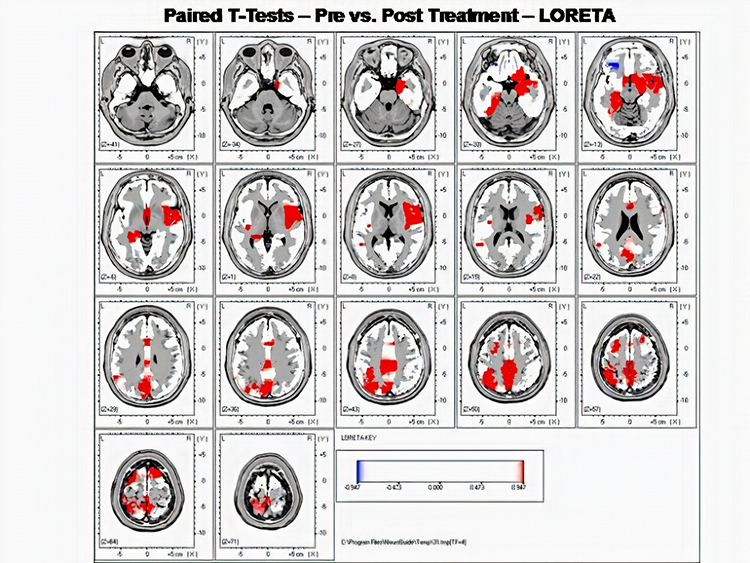
LORETA source localization across coronal, horizontal, and sagittal slices. Graphic courtesy of BrainMaster Technologies.
Standardized LORETA
Standardized LORETA (sLORETA) and eLORETA partition the intracerebral volume into 6,239 voxels at 5 mm resolution, refining the original LORETA's 2,394 voxels at 7 mm. Note that voxel size is not the same as spatial resolution: all LORETA-family solutions produce blurred images whose point-spread is on the order of centimeters, which is why sLORETA's effective resolution is often quoted as roughly one cubic centimeter even though its voxels are 5 mm on a side. sLORETA estimates each voxel's electrical potential without regard to frequency, and its values are expressed in normalized F values.
This refinement trades absolute units of current density for reduced noise and more precise source localization. The trade matters because LORETA's "three-sphere model," which assumes different conductivity for cortex, skull, and skin, suffers from artifacts sometimes called ghost images, along with limited source localization (Thompson & Thompson, 2015).
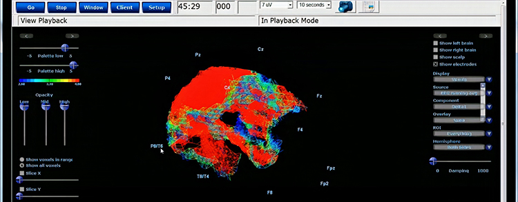
Standardized LORETA (sLORETA) source localization. Graphic courtesy of BrainMaster Technologies.
Exact LORETA
A third version of LORETA, eLORETA, exact low resolution brain electromagnetic tomography, has the property of exact, zero-error localization for a single point source, and it retains zero localization bias under specific noise assumptions (Pascual-Marqui, 2007). That does not mean it localizes multiple or spatially distributed sources without error, and the reconstruction remains blurred (Thompson & Thompson, 2015). Treat a zero-error claim carefully: it is a property of the mathematics under stated conditions, not a guarantee about the record sitting on your screen.
Variable Resolution Electromagnetic Tomography
The LORETA line is not the only inverse solution in clinical use. Variable resolution electromagnetic tomography (VARETA) is a source-space z-score method developed by Bosch-Bayard and colleagues (2001) that has shown high sensitivity and specificity. VARETA differs from LORETA in an instructive way: rather than imposing one smoothness constraint everywhere, it applies a probabilistic anatomical mask that lets the smoothness of the inverse solution vary from place to place. The practical consequence is that VARETA estimates distributed and discrete sources with roughly equal accuracy, whereas LORETA's uniform smoothing favors distributed ones (Thatcher & Lubar, 2009).
That property matters when a generator is genuinely focal. Machado and colleagues (2004) used VARETA to characterize acute middle cerebral artery ischemic stroke, a condition in which the abnormality is anatomically circumscribed and a solution biased toward smooth, distributed activity would tend to blur it away.
Weighted LORETA and Subcortical Solution Spaces
Standardized weighted LORETA (swLORETA) applies depth weighting to the inverse solution so that deeper generators are not systematically underestimated, which allows the solution space to be extended below the cortical surface. NeuroGuide implements swLORETA in its NeuroNavigator imaging feature using 12,400 voxels, and its solution space includes structures absent from classic LORETA, among them the cerebellum, red nucleus, nucleus accumbens, and habenula. NeuroNavigator also reports a phase slope index used to infer the direction of information flow between regions (Thatcher et al., 2020).
Read those subcortical images with the same discipline you apply to cortical ones. Extending the solution space changes what the algorithm is permitted to report; it does not add information to a 19-channel recording. Deep structures remain far from the sensors, their contribution to the scalp field is small, and depth weighting recovers them only under the assumptions built into the head model. A subcortical maximum in a swLORETA image is a hypothesis worth noting, not a measurement of thalamic or limbic activity in the sense an intracranial electrode would provide.
Source-Space Normative Databases and z-Scores
An inverse solution by itself tells you the estimated current density at a voxel. It does not tell you whether that value is unusual. Source-space normative databases close that gap by referencing each voxel to an age-matched normative sample and expressing the result as a z-score, the same logic that governs surface qEEG metrics but applied in three dimensions.
Thatcher and colleagues (2005) developed and evaluated a normative database for LORETA, reporting good cross-validation results and sensitivity relative to surface EEG measures, and Hoffman (2006) found high accuracy when that database was applied to patients carrying a range of neurological diagnoses. Thatcher, Biver, and North (2007) then extended the approach to spatial-temporal current source correlations, which allows connectivity to be assessed between voxels rather than between scalp channels. Pascual-Marqui and colleagues (2001) had earlier used LORETA for both functional localization and functional connectivity in first-episode, drug-naive patients with schizophrenia compared with normal controls, an early demonstration that source-space metrics could distinguish clinical groups.
Real-time applications require a z-score that updates continuously rather than one computed over an epoch after the fact. That is accomplished with joint time-frequency analysis (JTFA), which uses complex demodulation to produce a nearly instantaneous estimate of power in a band, from which a z-score is calculated moment by moment. This is the computational basis of surface and sLORETA z-score neurofeedback. One property of JTFA deserves emphasis: it yields smaller z-scores than the conventional FFT calculation, so it produces a more conservative estimate of how far a value deviates from the normative sample (Thatcher & Lubar, 2009).
Reliability is the obvious question to ask of any metric used for clinical decisions. Cannon and colleagues (2012) examined qEEG measures and LORETA current source density over a 30-day interval and found good test-retest stability, which supports the use of source-space metrics for tracking change across sessions rather than only within a single recording.
Two records taken six weeks apart show a drop in current density in a left frontal region. Before you attribute that change to the intervention, confirm that the two recordings used the same solution (LORETA, sLORETA, swLORETA, or VARETA are not interchangeable), the same normative database and age stratum, and comparable artifact rejection. Because Cannon and colleagues (2012) established 30-day stability for these measures, a shift that exceeds ordinary test-retest variation is interpretable. A shift that does not exceed it is noise wearing the costume of progress.
Laplacian Analysis
Surface Laplacian (SL) analysis, also called current source density (CSD) and scalp current density (SCD), is a family of mathematical algorithms that produce two-dimensional images of radial current flow from cortical dipoles to the scalp. Positive values represent current flowing from the cortex to the scalp, which are sources. Negative values represent current flowing from the scalp toward the brain, which are sinks.
Unlike the LORETA family of inverse solutions, SL analysis is independent of the reference recording procedure. Every reference scheme will yield the same current flow estimates and the same polarity, which removes an entire category of interpretive argument.
SL analysis also localizes the EEG signal better than surface potentials do, because it minimizes the scalp EEG blurring produced by volume conduction. Unlike inverse solutions, SL requires no model of the sources and is relatively insensitive to the volume conductor model. Kayser and Tenke (2015) put the point concretely: the surface Laplacian makes no assumptions about differences in tissue conductivity, about functional neuroanatomy, about cortical geometry and shape, or about the number and configuration of EEG sources. Every one of those is an assumption an inverse solution must make before it can return a single voxel value.
It is not, however, assumption-free. The standard spherical spline implementation assumes an idealized head geometry onto which electrode positions are projected, requires the analyst to choose a spline flexibility parameter and a regularization constant, and depends on adequate spatial sampling. Dense arrays of 64 or more electrodes give substantially better estimates than a 19-channel montage (Kayser & Tenke, 2015).
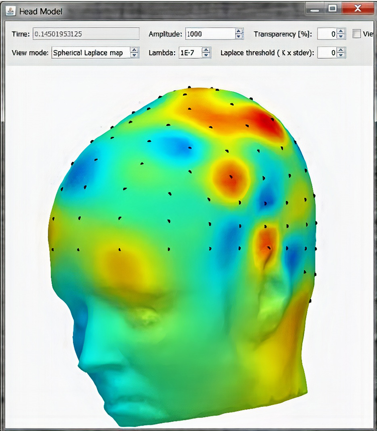
Surface Laplacian map of radial current flow. This figure was uploaded by Zoltan Juhasz to ResearchGate.
Color maps, contour plots, 3D surface plots, and time-series plots each answer a different question about the same data: how much, where exactly, how the surface is shaped, and when. The LORETA family solves the inverse problem to estimate cortical generators, assigning voxels Talairach coordinates that transfer across PET and MRI, with sLORETA and eLORETA partitioning the volume into 6,239 voxels at 5 mm and eLORETA achieving exact, zero-error localization for a single point source. Voxel size is not spatial resolution, and every LORETA-family image stays blurred at the scale of centimeters. The classic LORETA and sLORETA solution spaces are restricted to cortical gray matter and therefore cannot resolve subcortical structures; VARETA relaxes the uniform smoothness constraint with a probabilistic mask, and swLORETA applies depth weighting to extend the solution space to structures such as the cerebellum and nucleus accumbens, but neither adds information to a 19-channel recording. Source-space normative databases convert voxel values into z-scores, JTFA supplies the near-instantaneous z-scores used in real-time neurofeedback at a deliberately conservative magnitude, and these measures show good 30-day test-retest stability. Surface Laplacian analysis reaches a related goal by a different route: it is reference-free and needs no model of the sources, tissue conductivity, functional neuroanatomy, or cortical geometry, though it still assumes an idealized head geometry and depends on adequate spatial sampling.
A client is referred to you after a mild traumatic brain injury, and the referring clinician's report states that a 19-channel LORETA image shows thalamic dysregulation. You should pause here. LORETA solutions built from 19 scalp electrodes estimate cortical generators only, so a thalamic claim exceeds what the method can support. Ask which solution actually produced the image, because a depth-weighted variant such as swLORETA does place voxels in selected subcortical structures, and a value reported from such a voxel is a model-dependent estimate rather than a direct measurement. A more defensible reading describes the cortical maxima by Brodmann area and Talairach coordinate, names the inverse solution and normative database, notes the reference montage used, and states the resolution limit explicitly. If reference dependence is a concern in that record, a surface Laplacian map offers a useful cross-check, because its current flow estimates and polarity will be identical no matter which reference the original recording used.
Check Your Understanding
- Which graphic method would you choose to demonstrate the exact boundary of a region of elevated current density, and why?
- What does the “owl eye” appearance in a topographic color map indicate about the underlying rhythm?
- How do LORETA, sLORETA, and eLORETA differ in spatial resolution, units of measurement, and claimed localization error?
- Why can Talairach coordinates be shared across EEG, PET, and MRI studies?
- How does VARETA's probabilistic mask change what the inverse solution can recover, and why did that matter in the stroke work of Machado and colleagues?
- swLORETA reports voxels in the cerebellum and nucleus accumbens. What exactly has been added relative to sLORETA, and what has not?
- Why does the JTFA z-score used in real-time neurofeedback run smaller than the FFT-based z-score, and is that a problem?
- Name two assumptions that inverse solutions require and that surface Laplacian analysis avoids, and two assumptions the surface Laplacian still makes.
Applications of CSD Analysis
CSD analysis is widely used in both basic and clinical neuroscience research. In basic research, it helps to elucidate the mechanisms of sensory processing, cognitive functions, and neural oscillations.
In clinical settings, CSD analysis can aid in the diagnosis and treatment of neurological disorders by providing detailed maps of brain activity that are simply not accessible through traditional EEG or LFP recordings (Kayser & Tenke, 2006). The clinical payoff is specificity: a finding tied to a location and a time course is far easier to act on than a finding tied to a channel label.
Taken together, CSD analysis offers detailed insight into the spatial and temporal patterns of neural activity. By using metrics such as source strength, distribution, and dynamics, and by employing the graphic methods described in this unit, you can build a deeper understanding of brain function and dysfunction. Continued development of these techniques promises to advance our knowledge of the brain and to improve clinical outcomes.
CSD analysis serves basic research by clarifying sensory processing, cognition, and neural oscillations, and it serves clinical work by producing activity maps that raw EEG and LFP recordings cannot deliver. Its value in the clinic comes from specificity, because a finding anchored to a location and a time course supports action in a way that a channel label does not. Used together, the three metrics and the four graphic methods let you describe how strong an effect is, where it sits, and when it unfolds.
Cutting-Edge Topics in qEEG Research
Reference-Free Spectra and Frequency Principal Components Analysis
One of the oldest embarrassments in quantitative EEG is that the numbers change when the reference changes. Tenke, Kayser, and Murray (2015) addressed this directly by combining current source density with frequency principal components analysis to produce reference-free quantification of EEG spectra. The appeal is practical rather than theoretical: two laboratories using different references can compare results without arguing about montage.
The approach also compresses the frequency dimension empirically instead of relying on fixed band boundaries. That matters because the traditional delta, theta, alpha, and beta cut points are conventions, not facts about any individual brain.
Millisecond-Scale Mapping of Early Sensory Responses
Poghosyan and Ioannides (2007) demonstrated precise mapping of early visual responses in both space and time, which is exactly the combination that CSD methods are built to deliver. Their work illustrates why source dynamics deserves equal billing with source strength and distribution. A response that is 20 milliseconds early tells you something a static map never will.
This line of work continues to push toward finer temporal windows in sensory and cognitive research, where the sequence of activation, rather than its amplitude, carries the theoretical weight.
From Cortical Laminae to the Scalp
The foundations of CSD were laid in laminar recordings, where Nicholson and Freeman (1975) developed the theory and conductivity tensor for the anuran cerebellum and Mitzdorf (1985) applied the method to cat cerebral cortex. Those studies established that sinks and sources map onto identifiable synaptic events within cortical layers.
Current research asks how much of that laminar specificity survives the trip to the scalp. High-density arrays and improved head models are narrowing the gap, but the honest answer is still that scalp CSD estimates a smoothed version of what a laminar probe would see.
Laplacian Waveforms as Input to Connectivity and Classification
Kayser and Tenke (2006) showed that principal components analysis of Laplacian waveforms identifies event-related potential generator patterns in a generic, task-independent way. That result has an important downstream consequence: because Laplacian transformation removes reference dependence and reduces volume conduction, it makes a better input to connectivity metrics and machine-learning classifiers than raw surface potentials do.
Expect to see more studies that apply a surface Laplacian as a routine preprocessing step before computing coherence, phase measures, or classifier features. Cleaning the spatial signal first is cheaper than correcting for volume conduction afterward.
Assignment
Now that you have completed this unit, explain how eLORETA can enhance source localization. In your answer, state what problem in the earlier LORETA and sLORETA solutions eLORETA was designed to address, describe what the claim of zero localization error does and does not promise, and identify one limitation that no 19-channel inverse solution can overcome.
Glossary
3D surface plots: three-dimensional representations of qEEG data in which the height of the surface corresponds to the magnitude of current density, providing a detailed view of the spatial distribution of neural activity.
color maps: visual representations of qEEG data in which different colors indicate varying magnitudes of brain activity or current density, allowing intuitive interpretation of complex data.
contour plots: graphs that use lines to represent areas of equal current density or activity in qEEG data, similar to topographic maps, used to visualize the spatial structure of neural activity.
current sink: a region of inward positive transmembrane current that produces relative negativity in the surrounding extracellular field.
current source density (CSD) mapping: a topographic display of the local current sources and sinks estimated at each scalp site from the surface Laplacian of the voltage field, sharpening spatial detail.
exact low-resolution brain electromagnetic tomography (eLORETA): a third-generation refinement of LORETA with the property of exact, zero-error localization for a single point source, retaining zero localization bias under specific noise assumptions; it does not localize multiple or spatially distributed sources without error.
inverse problem: the challenge of estimating which cortical generators produced a recorded pattern of scalp voltages, given that many different source configurations can produce the same surface recording.
joint time-frequency analysis (JTFA): a family of techniques that analyze signals with time-varying frequency content, providing information in both the time and frequency domains and enabling real-time z-score training.
Laplacian analysis: a mathematical method used in qEEG to enhance spatial resolution by calculating the second spatial derivative of the EEG signal, effectively highlighting local sources of brain activity.
local field potential (LFP): a low-frequency extracellular voltage reflecting summed transmembrane currents from a local neural population, especially synaptic and dendritic activity.
low-resolution electromagnetic tomography (LORETA): the inverse solution of Pascual-Marqui and colleagues (1994) that estimates three-dimensional cortical sources of scalp-recorded EEG at low spatial resolution.
source: the place at the end of the neuron opposite the sink where current leaves, making the surrounding extracellular area electrically positive.
source distribution: the spatial extent and pattern of current sources and sinks in the brain, providing information about the localization and spread of neural activity.
source dynamics: the moment-to-moment changes in estimated current density that reveal the timing and sequence of neural events.
source strength: a measure of the magnitude of current sources and sinks in the brain, expressed in units of current density (A/m²), indicating the intensity of neuronal activity.
source-space normative database: a normative reference sample that expresses estimated current density at each voxel as a z-score relative to age-matched healthy participants, extending the logic of surface qEEG norms into three dimensions and providing the basis for LORETA and sLORETA z-score neurofeedback.
standardized low-resolution brain electromagnetic tomography (sLORETA): a variation of LORETA that partitions the intracerebral volume into 6,239 voxels at 5 mm resolution, standardizes current density values, and expresses them as normalized F values, improving the statistical reliability and localization accuracy of brain activity sources.
standardized weighted low-resolution brain electromagnetic tomography (swLORETA): a depth-weighted refinement of sLORETA that compensates for underestimation of deep generators, extending the solution space below the cortex to the thalamus and cerebellum. Extending the solution space changes what the algorithm may report, not what a 19-channel recording contains.
surface Laplacian (SL) analysis: a family of mathematical algorithms that provide two-dimensional images of radial current flow from cortical dipoles to the scalp.
Talairach coordinate: a three-axis Cartesian coordinate whose origin is the anterior commissure, with the y-axis along the AC-PC line, the z-axis inferior-to-superior, and the x-axis left-to-right; expressed in millimeters as (x, y, z) and referenced to the Talairach or Montreal atlases.
time-series plots: graphs that display the temporal evolution of EEG or qEEG data at specific locations or across the entire electrode array, used to analyze the dynamics of brain activity over time.
variable resolution electromagnetic tomography (VARETA): a z-score inverse solution that applies a probabilistic anatomical mask, allowing the smoothness of the solution to vary across the brain rather than being fixed, so that distributed and discrete sources are estimated with comparable accuracy.
volume conduction: passive spread of electrical fields through conductive biological tissues, allowing a source to influence electrodes located at a distance.
voxel: a three-dimensional pixel representing a volumetric element in neuroimaging data such as qEEG or MRI, used to localize and quantify brain activity within a specific region.
Test Yourself on ClassMarker
Click the button below to take a 10-question exam over this entire unit. There is no password.
Review Flash Cards on Quizlet
Click the button below to review our chapter flash cards.
References
Bosch-Bayard, J., Valdés-Sosa, P., Virues-Alba, T., Aubert-Vázquez, E., John, E. R., Harmony, T., Riera-Díaz, J., & Trujillo-Barreto, N. (2001). 3D statistical parametric mapping of EEG source spectra by means of variable resolution electromagnetic tomography (VARETA). Clinical Electroencephalography, 32(2), 47-61. https://doi.org/10.1177/155005940103200203
Cannon, R. L., Baldwin, D. R., Shaw, T. L., Diloreto, D. J., Phillips, S. M., Scruggs, A. M., & Riehl, T. C. (2012). Reliability of quantitative EEG (qEEG) measures and LORETA current source density at 30 days. Neuroscience Letters, 518(1), 27-31. https://doi.org/10.1016/j.neulet.2012.04.035
Freeman, J. A., & Nicholson, C. (1975). Experimental optimization of current source-density technique for anuran cerebellum. Journal of Neurophysiology, 38(2), 369-382. https://doi.org/10.1152/jn.1975.38.2.369
Hoffman, D. (2006). LORETA: An attempt at a simple answer to a complex controversy. Journal of Neurotherapy, 10(1), 57-72. https://doi.org/10.1300/J184v10n01_05
Kayser, J., & Tenke, C. E. (2006). Principal components analysis of Laplacian waveforms as a generic method for identifying ERP generator patterns: I. Evaluation with auditory oddball tasks. Clinical Neurophysiology, 117(2), 348-368. https://doi.org/10.1016/j.clinph.2005.08.034
Kayser, J., & Tenke, C. E. (2015). On the benefits of using surface Laplacian (current source density) methodology in electrophysiology. Int J Psychophysiol, 97(3), 171-173. https://dx.doi.org/10.1016%2Fj.ijpsycho.2015.06.001
Machado, C., Cuspineda, E., Valdés, P., Virues, T., Llopis, F., Bosch, J., Aubert, E., Hernández, E., Pando, A., Alvarez, M. A., Barroso, E., Galán, L., & Avila, Y. (2004). Assessing acute middle cerebral artery ischemic stroke by quantitative electric tomography. Clinical EEG and Neuroscience, 35(3), 116-124. https://doi.org/10.1177/155005940403500303
Mitzdorf, U. (1985). Current source-density method and application in cat cerebral cortex: Investigation of evoked potentials and EEG phenomena. Physiological Reviews, 65(1), 37-100. https://doi.org/10.1152/physrev.1985.65.1.37
Nicholson, C., & Freeman, J. A. (1975). Theory of current source-density analysis and determination of conductivity tensor for anuran cerebellum. Journal of Neurophysiology, 38(2), 356-368. https://doi.org/10.1152/jn.1975.38.2.356
Pascual-Marqui, R. D. (2007). Discrete, 3D distributed, linear imaging methods of electric neuronal activity. Part 1: Exact, zero error localization. arXiv:0710.3341 [math-ph]. https://arxiv.org/abs/0710.3341
Pascual-Marqui, R. D., Koukkou, M., Lehmann, D., & Kochi, K. (2001). Functional localization and functional connectivity with LORETA comparison to normal controls and first episode drug naive schizophrenics. Journal of Neurotherapy, 4(4), 35-37. https://doi.org/10.1300/J184v04n04_06
Pascual-Marqui, R. D., Michel, C. M., & Lehmann, D. (1994). Low resolution electromagnetic tomography: A new method for localizing electrical activity in the brain. International Journal of Psychophysiology, 18(1), 49-65. https://doi.org/10.1016/0167-8760(84)90014-X
Poghosyan, V., & Ioannides, A. A. (2007). Precise mapping of early visual responses in space and time. NeuroImage, 35(2), 759-770. https://doi.org/10.1016/j.neuroimage.2006.11.052
Tenke, C. E., Kayser, J., & Murray, M. M. (2015). Reference-free quantification of EEG spectra: Combining current source density (CSD) and frequency principal components analysis (fPCA). Clinical Neurophysiology, 126(12), 2324-2337. https://doi.org/10.1016/j.clinph.2015.03.012
Thatcher, R. W., Biver, C. J., & North, D. (2007). Spatial-temporal current source correlations and cortical connectivity. Clinical EEG and Neuroscience, 38(1), 35-48. https://doi.org/10.1177/155005940703800109
Thatcher, R. W., Biver, C. J., Soler, E. P., Lubar, J., & Koberda, J. L. (2020). New advances in electrical neuroimaging, brain networks, and neurofeedback protocols. Journal of Neurology and Neurobiology, 6(1), 1-14. https://doi.org/10.16966/2379-7150.168
Thatcher, R. W., & Lubar, J. F. (2009). History of the scientific standards of qEEG normative databases. In T. H. Budzynski, H. K. Budzynski, J. R. Evans, & A. Abarbanel (Eds.), Introduction to quantitative EEG and neurofeedback: Advanced theory and applications (2nd ed., pp. 29-59). Academic Press.
Thatcher, R. W., North, D., & Biver, C. J. (2005). Evaluation and validity of a LORETA normative EEG database. Clinical EEG and Neuroscience, 36(2), 116-122. https://doi.org/10.1177/155005940503600211
Thompson, M., & Thompson, L. (2015). The neurofeedback book: An introduction to basic concepts in applied psychophysiology (2nd ed.). Association for Applied Psychophysiology and Biofeedback.
Return to Top