Instrumentation: Acquisition and Review Parameters

Learning Objectives

After completing this section, you will be able to:

Acquisition and Review Parameters

Quantitative Electroencephalography (qEEG) is a powerful tool in neuropsychology and neuroscience for analyzing the brain's electrical activity. Ensuring accurate and reliable data collection involves several critical parameters and settings.

Listen to the Full-Length Lecture

First, electrode placement and the number of electrodes are fundamental. Standardized placement using the International 10-20 or 10-10 system is essential for consistent and reproducible electrode locations across subjects and sessions (Klem et al., 1999). Typically, a high-density cap with 19, 32, 64, or more electrodes captures detailed spatial information (Nuwer, 1997).

Second, the sampling rate is another crucial parameter. The minimum sampling rate should be at least 256 Hz, but higher rates, such as 512 Hz or 1024 Hz, are preferred for capturing fast neural dynamics and avoiding aliasing (Miller et al., 2009).

Third, data acquisition settings also play a vital role. Filter settings should include a high-pass filter set around 0.5-1 Hz and a low-pass filter set around 70-100 Hz to remove artifacts and noise outside the frequency range of interest (Luck, 2014). A 50/60 Hz notch filter should also be applied to eliminate power line noise, depending on the regional electrical supply frequency.

Fourth, maintaining low impedance levels is essential for signal quality. Electrode impedances should be kept below 5 kΩ to ensure good signal quality and reduce artifacts, with lower impedance values preferable (Ferree et al., 2001).

Fifth, artifact management is another critical aspect of qEEG. Implementing real-time artifact rejection algorithms can help exclude segments contaminated by eye movements, muscle activity, or electrical noise. Post-processing methods, such as Independent Component Analysis (ICA), are useful for artifact correction (Jung et al., 2000).

Sixth, the choice of reference electrode can significantly affect the results. Common references include linked earlobes, mastoids, or an average reference, and this choice should be consistent across subjects and sessions (Yao, 2001).

Seventh, the recording environment should be controlled to minimize environmental noise and ensure subject comfort. This includes performing recordings in a quiet, electrically shielded room with controlled temperature and lighting.

Finally, proper subject preparation is essential for accurate qEEG data. Subjects should avoid caffeine, heavy meals, and intense physical activity before the recording session. Ensuring they are well-rested and relaxed can help reduce movement artifacts.

These settings and parameters are critical for obtaining high-quality qEEG data, which can provide valuable insights into brain function and dysfunction.

EEG Filters Define the Signal

EEG filters select signals of interest and minimize artifacts. This section reviews high-pass, low-pass, bandpass, and notch filters—the tools your equipment uses to isolate the frequency bands that matter for clinical decision-making.

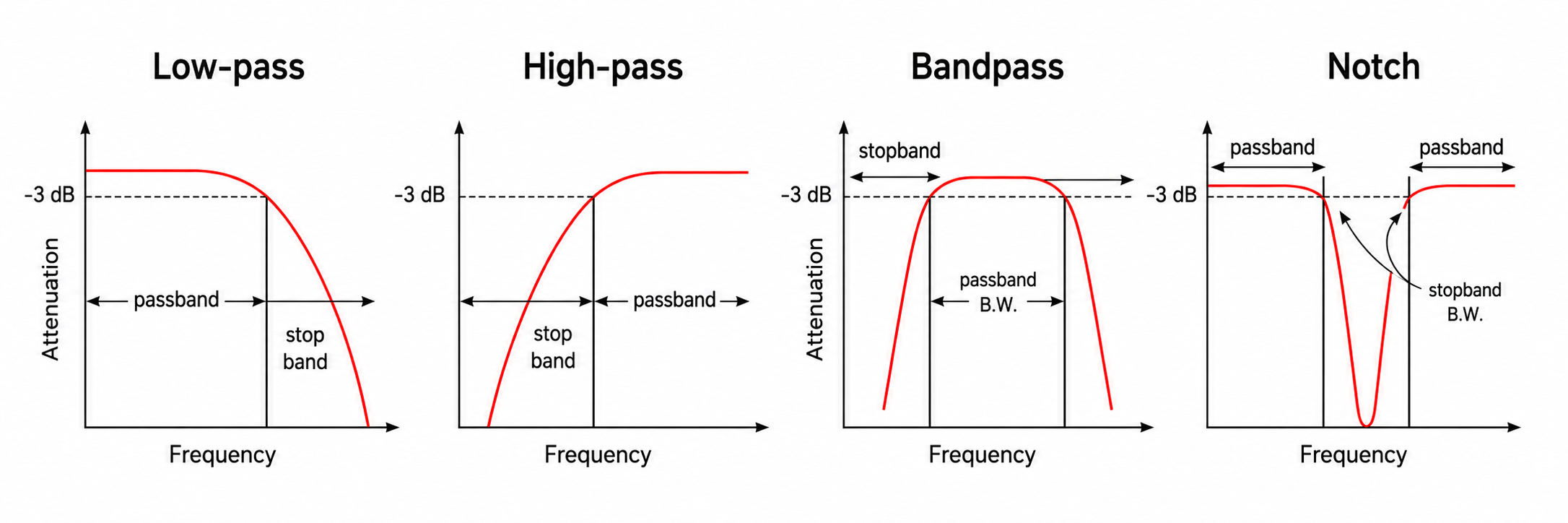
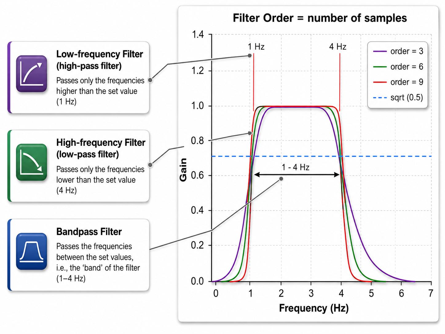
The range of frequencies passed through a filter is called the passband, and the range sharply attenuated is called the stopband. A high-pass filter only passes frequencies above a set value (e.g., 1 Hz), while a low-pass filter only passes frequencies below a specified value (e.g., 40 Hz). A bandpass filter combines both, passing only the frequencies between the set values—the "band" of the filter (e.g., 1-40 Hz).

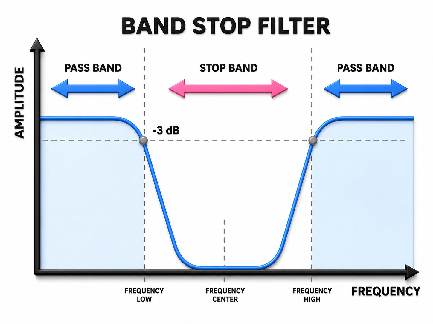
A notch filter reverses the arrangement of passbands and stopbands found in a bandpass filter. Instead of passing a narrow band of frequencies, it attenuates a narrow window, or "notch," while allowing frequencies above and below it to pass. Notch filters commonly target mains interference at 60 Hz in North America and 50 Hz in most other regions. (See the discussion of notch filters below.)

Filter Order

A filter's precision depends on how many data points it uses to define the boundary between the signal it passes and the signal it blocks. Lower-order filters use fewer data points, define that boundary less sharply, and roll off gradually between the frequencies they stop and the frequencies they pass. Higher-order filters use more data points and produce a more sharply defined boundary. That added sharpness comes at a cost, because processing more data points delays the filter's output. Neurofeedback providers therefore typically use filter orders between 3 and 6, balancing a well-defined boundary against acceptable delay.

The following movies demonstrate the effects of low-pass and high-pass filters at various settings.

10-Hz Low-Pass Filter

The movie below shows the output of a 10-Hz low-pass filter with a vertical scale of 0-50 μV © John S. Anderson.

20-Hz Low-Pass Filter

The movie below shows the output of a 20-Hz low-pass filter with a vertical scale of 0-50 μV © John S. Anderson.

30-Hz Low-Pass Filter

The movie below shows the output of a 30-Hz low-pass filter with a vertical scale of 0-50 μV © John S. Anderson.

40-Hz Low-Pass Filter

The movie below shows the output of a 40-Hz low-pass filter with a vertical scale of 0-50 μV © John S. Anderson.

10-Hz High-Pass Filter

The movie below shows the output of a 10-Hz high-pass filter with a vertical scale of 0-50 μV © John S. Anderson.

20-Hz High-Pass Filter

The movie below shows the output of a 20-Hz high-pass filter with a vertical scale of 0-50 μV © John S. Anderson.

30-Hz High-Pass Filter

The movie below shows the output of a 30-Hz high-pass filter with a vertical scale of 0-50 μV © John S. Anderson.

Bandpass Filters

1-40-Hz Bandpass Filter

The movie below shows the output of a 1-40-Hz bandpass filter with a vertical scale of 0-50 μV © John S. Anderson.

8-12-Hz Bandpass Filter

The movie below shows the output of an 8-12-Hz bandpass filter with a vertical scale of 0-50 μV © John S. Anderson.

The movie below shows the output of three bandpass filters for delta, theta, and alpha © John S. Anderson.

The movie below generously provided by John S. Anderson shows a "raw" or "wave" display of oscillating electrical information using a positive/negative scale with 0.0 in the middle with the voltage displayed as peak-to-peak μV.

The movie © John S. Anderson shows the same alpha waveform plotted along two scales. The top display plots the waveform on a scale from -20 to +20 μV, while the bottom "amplitude" display plots the voltage on a scale from 0-50 μV where all values are positive.

The movie © John S. Anderson shows the conversion of the complex EEG signal into its spectral components.

The movie © John S. Anderson shows the spectrum magnitude (average amplitude over a given time) in the top display and power (μV²) in the bottom display.

The movie © John S. Anderson shows the same alpha activity displayed in terms of amplitude (positive voltages), power or amplitude² (picowatts/resistance), and percent power (signal power as a percentage of total EEG power from 0-100%).

Notch Filter

A notch filter suppresses a narrow band of frequencies produced by line current (e.g., 50/60 Hz artifact). The stopband is the range of frequencies attenuated by the notch filter. Use notch filters as a last resort because they remove all signal energy at the target frequency, not just artifact—meaning genuine EEG activity at 50/60 Hz is also eliminated.

The narrated video below © John S. Anderson displays the same 21-channel recording viewed using different montages with a 60-Hz notch filter on and off.

Digital Filters

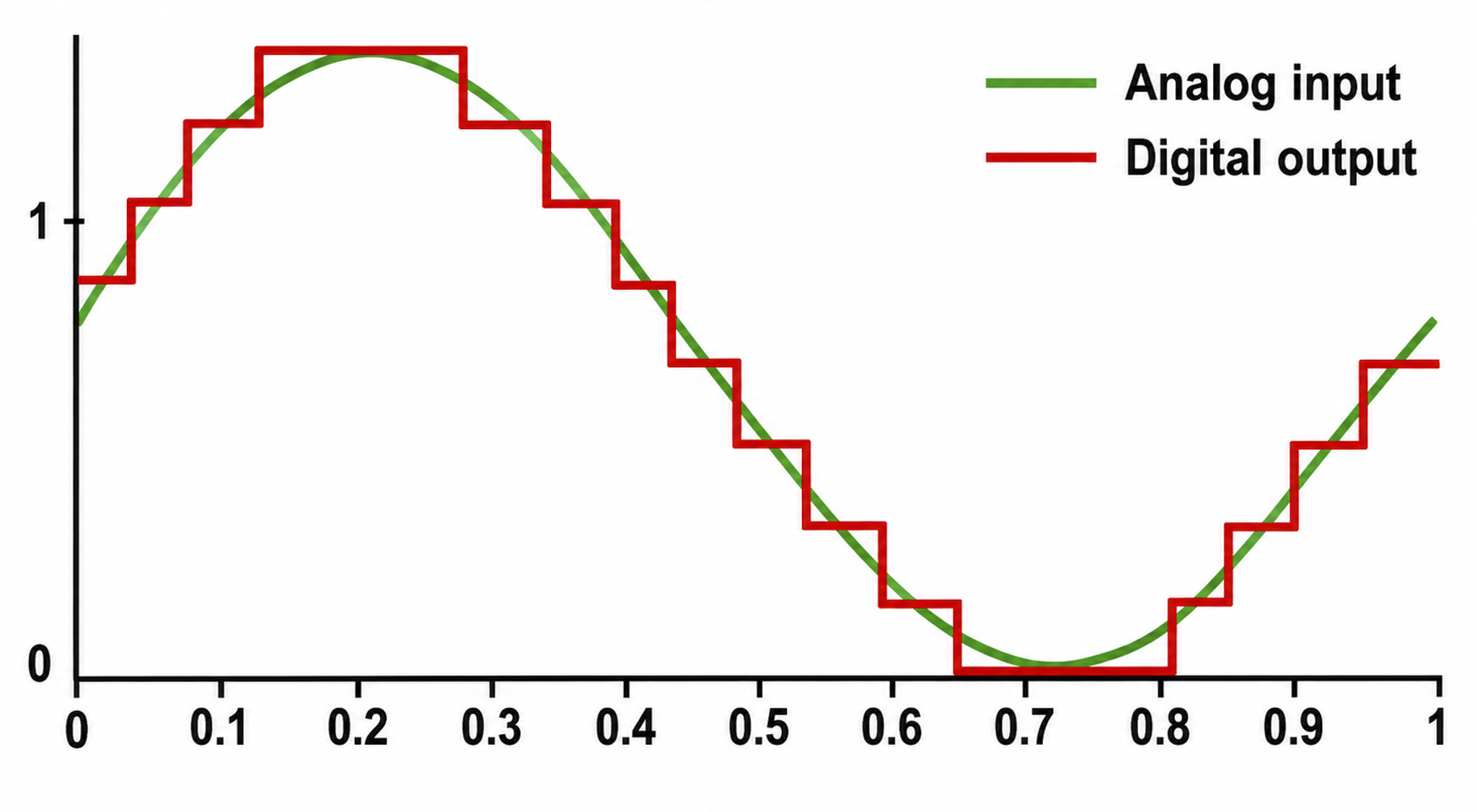
Digital filters use digital processors, like a digital signal processing (DSP) chip, to exclude unwanted frequencies. The process has three steps: first, an analog-to-digital converter (ADC) samples and digitizes the analog signal, representing signal voltages as binary numbers; second, a DSP chip performs calculations on those binary numbers; and third, a digital-to-analog converter (DAC) may transform the sampled, digitally-filtered signal back to analog form.

Three main methods of digital filtering are used in EEG systems. FFT (Fast Fourier Transformation) filters convert the EEG signal into a set of sine waves varying in frequency, amplitude, and phase. FIR (finite impulse response) filters have a finite-duration impulse response and calculate a moving weighted average of digitally sampled voltages. IIR (infinite impulse response) filters employ feedback to calculate a moving weighted average of digitally sampled voltages.

All three methods share four advantages over analog filters. First, clinicians can retrospectively adjust filter settings while reviewing the EEG record since digital filters are programmable. Second, digital filters can be designed to minimize phase distortion—the displacement of the EEG waveform in time. Third, they are stable over time and across a range of temperatures. Fourth, they accurately process low-frequency signals.

An important caveat: since these three digital filtering methods can yield different statistical values, they cannot be used interchangeably. Only compare FFT statistics with other FFT statistics—never with FIR or IIR results (Thompson & Thompson, 2015). Mixing methods can lead to misleading comparisons and flawed clinical conclusions.

Below is a BioGraph ® Infiniti EEG three-dimensional FFT display. Frequency is displayed on the X-axis, amplitude on the Y-axis, and time on the Z-axis.

What an FFT Display Shows You

An FFT converts the raw EEG into frequency and magnitude, which is the amplitude of each frequency component averaged over the analyzed interval (Anderson, 2025). Where the raw tracing presents voltage on the y-axis and time on the x-axis as one undifferentiated line, the FFT display places frequency on the x-axis and magnitude on the y-axis, so the single frequencies that make up each band become visible individually. Systems typically color-code these collections as delta (1-4 Hz), theta (4-8 Hz), alpha (8-12 Hz), the sensorimotor rhythm (SMR) at 12-15 Hz, also called beta 1, low beta (15-22 Hz, or beta 2), middle beta (22-36 Hz, or beta 3), and high beta (36-45 Hz, also called beta 4 or gamma), with the caution that these designations vary slightly from one system to another (Anderson, 2025).

This arrangement lets you see at a glance how much activity occupies each band, which is the information you need when selecting a reward bandwidth. It also displays the peak frequency, the frequency carrying the highest voltage within a given band, such as 10 Hz within an 8-12 Hz alpha band, and many displays print the mean, median, and dominant frequency as text alongside the graph (Anderson, 2025). Because reward and inhibit bands are most effective when centered on where a client's activity actually lives rather than on a textbook range, reading the peak frequency before setting bandwidths is a small step that meaningfully improves protocol fit.

Resolution can be finer than whole bands. Depending on software and hardware, the spectrum can be examined in 0.5-Hz segments or smaller, though the more common practice is to inspect 1-Hz frequency bins, meaning narrow frequency slices analyzed one at a time (Anderson, 2025). Bin-level inspection is how distinctive features are found. The mu rhythm, an 8-12 Hz rhythm generated over the sensorimotor cortex that is suppressed by movement and by observing movement, is usually isolated by its location and its frequency bin rather than by band labels alone (Anderson, 2025).

What an FFT Display Hides

The clarity of a spectral display comes at the expense of vital information. Once the data have been processed, it is impossible to know how much of the activity shown is genuine cortical signal and how much is artifact from eye movement or from muscle activity, which enters the recording as electromyography (EMG) (Anderson, 2025). In Anderson's example recording, a substantial eye artifact elevated the low-frequency voltage even though little EMG was present, because eye movements and blinks produce electrical discharges that fall within delta and low theta frequencies. Those discharges do not originate in the brain as EEG, yet they occupy the same frequencies and are plotted into the EEG graph as though they did (Anderson, 2025). The practical rule is that no spectral value, ratio, or z-score deserves your confidence until you have inspected the raw tracing that produced it and removed or excluded the contaminated segments.

Time resolution is the second casualty. A display calculated from 2 seconds of EEG is a composite of those 2 seconds and therefore loses the moment-by-moment detail visible in the raw display (Anderson, 2025). One second is the minimum window an FFT calculation requires, and the same computation can average across many minutes to represent typical activity over a longer period, which is what makes normative databases and topographic maps possible (Anderson, 2025). This trade-off should be a deliberate choice. Short epochs—the discrete time segments into which a recording is divided for analysis—keep feedback responsive enough for the client to perceive a contingency, while long averages give assessment values the stability that protocol decisions require. Values derived from different epoch lengths should not be compared as though they were equivalent.

From Amplitude to Power

Power means amplitude squared, so an amplitude of 4 μV corresponds to a power of 16 microvolts squared (μV²), which some systems label 16 picowatts because 1 μV² across a reference resistance of 1 ohm equals 1 pW (Anderson, 2025). Though the number differs from the amplitude value, it still represents the amount of electrical activity in the EEG. Squaring serves two purposes. The first is arithmetic: because the EEG constantly fluctuates between positive and negative values above and below the zero line, averaging the raw signal over time produces a result near zero, whereas squaring converts every value to a positive number so that means, maxima, minima, standard deviations, and other statistics can be calculated at all (Anderson, 2025).

The second purpose is visual differentiation. Squaring widens the apparent distance between bands, since 4 x 4 = 16 while 2 x 2 = 4, so a twofold difference in amplitude becomes a fourfold difference in power and the taller band becomes easier to identify at a glance (Anderson, 2025). The same recording plotted as a magnitude spectrum, which shows amplitude over time corrected for sign, and as a power spectrum, which shows amplitude squared, can carry y-axis scales as different as 0-12 μV and 0-96 pW while representing identical data (Anderson, 2025).

This has a direct and frequently overlooked consequence for ratio-based training. A theta/beta ratio comparing 4-8 Hz to 13-21 Hz reads 4/2, or 2.0, in amplitude terms and 16/4, or 4.0, in power terms for the very same brain (Anderson, 2025). A threshold borrowed from a colleague, a textbook, or a published study is therefore meaningless unless you know which convention produced it, and copying an amplitude-based ratio target into a power-based display will set your client an entirely different task than the one intended. Power values are also what normative databases use when computing z-scores, which express a client's value as a number of standard deviations (SD) from the database mean, with the interval from -1 to +1 SD containing roughly 68% of values in a normal distribution (Anderson, 2025).

Relative Power and the Illusion of Deficits

The other power value in common use travels under several names—relative power, percent power, and normalized EEG—that all refer to the same measurement (Anderson, 2025). Relative power converts the actual power values, known as absolute power, into percentages representing each band's power as a proportion of the power in the entire recorded band, and reports the result as a percentage. If the full 1-45 Hz band has a power value of 100 and 8-12 Hz has a power value of 25, then 8-12 Hz accounts for 25% of total EEG power (Anderson, 2025).

This transformation entered EEG analysis in its early days because the amplifiers of the era produced widely varying voltage values even when recording the same individual on different occasions. Converting to percentages promised to make any recording comparable to any other, which is why the results were called normalized EEG, and the measure remains in extensive use even in recently published research (Anderson, 2025).

The method carries a structural flaw that matters enormously at the point of protocol design. Because percentages must sum to 100, a single very high-amplitude band claims a disproportionately large share of the EEG "pie" and leaves every other frequency representing a smaller percentage than it deserves, which is especially treacherous when relative power values are compared against topographic z-score maps from a normative database (Anderson, 2025). Anderson's illustrative case makes the danger concrete. In the absolute power maps of that recording, 1 Hz and 2 Hz carried far more power than any other bin, and in relative power terms they accounted for 22.9% and 20.7% respectively, together consuming 43.6% of the entire pie. The absolute power z-score maps showed deviations up to +3 SD from 1-5 Hz and, critically, no blue regions anywhere, meaning no frequency bin was deficient at any location. The relative power z-score maps told a different story, showing negative values reaching -3 SD across 6-16 Hz in varying distributions.

Writing Protocols and Reports in Hertz

Terminology surrounding frequency and amplitude is a persistent source of confusion because the EEG is described with categorical terms like fast, slow, high, low, voltage, power, relative power, percent power, and amplitude, often interchangeably (Anderson, 2025). The band labels themselves have never been consistent. Beta frequencies between 24 and 36 Hz may be called high, fast, or beta 3, frequencies between 25 and 45 Hz may be called gamma or beta 4, and bands are further subdivided into alpha 1 and alpha 2 or beta 1 through beta 4 depending on the author. Amplitude adjectives then stack on top of frequency adjectives, producing constructions like high high beta, low high beta, high low alpha, and low low alpha, whose meaning is anyone's guess (Anderson, 2025). These inconsistencies have existed in electroencephalography from the beginning, which is itself the argument for abandoning the labels in favor of numbers.

Imprecision becomes costly at exactly the moment it matters most: when a practitioner reads an assessment report to determine a training protocol for a client (Anderson, 2025). A paper or report stating that there was "an increase in activity in the frontal EEG" leaves the reader unable to tell whether the increase occurred at 8-12 Hz, 15-18 Hz, or 4-8 Hz, and if the statement merely describes a general rise in voltage, its useful information approaches zero (Anderson, 2025). The remedy is to identify the EEG by the frequency under discussion—8-10 Hz rather than alpha 1, 24-36 Hz rather than beta 3, 36-44 Hz rather than beta 4 or gamma—so that everyone knows precisely what is meant (Anderson, 2025).

Consider the difference a precise sentence makes. A report might state that an increase in 4-8 Hz amplitude from 4 μV to 6 μV was noted in the prefrontal cortex, the anterior region of the frontal lobes that supports executive function and cognitive control, during an active memory recall task. Because abnormally high amplitude in that frequency range over prefrontal areas is associated with reduced cognitive performance, this description supports specific inferences: that the person disengaged during the task, or that the prefrontal cortex exerted less-than-normal cognitive control during it, among other possibilities (Anderson, 2025). Combined with behavioral information such as the client's degree of success on the task and findings from other testing, these data identify the specific location and frequency that correlate with the presenting concern and lead directly to a protocol. If elevated 4-8 Hz amplitude over prefrontal cortex accompanies lower memory scores, training to decrease prefrontal 4-8 Hz becomes a defensible candidate for improving memory (Anderson, 2025).

Categorical shorthand will not disappear, and it exists because it makes conversation easier. When a colleague remarks that "that alpha is really high," however, the statement could mean high amplitude, high-frequency alpha, or a high peak alpha frequency, and the best response is simply to ask which (Anderson, 2025). Language is a dynamic function and ambiguity in casual speech is tolerable, but precise terminology is not optional when writing for publication or preparing clinical reports. All of this counsels careful assumptions, precise language, and caution in how we approach a client's training, and it is worth remembering that EEG analysis, whether visual or quantitative, is a process that grows more accurate as our skills develop and our understanding of this elegant and information-rich measure deepens (Anderson, 2025).

Assignment

Now that you have completed this unit, describe the acquisition and review settings you would specify for a 19-channel eyes-closed recording, and justify each one. Then explain what you would lose if a colleague handed you the same recording collected at 128 Hz with a 30 Hz low-pass filter already applied, and whether any of it could be recovered.

Glossary

References

Ferree, T. C., Luu, P., Russell, G. S., & Tucker, D. M. (2001). Scalp electrode impedance, infection risk, and EEG data quality. Clinical Neurophysiology, 112(3), 536-544. https://doi.org/10.1016/s1388-2457(00)00533-2

Jung, T. P., Makeig, S., Humphries, C., Lee, T. W., McKeown, M. J., Iragui, V., & Sejnowski, T. J. (2000). Removing electroencephalographic artifacts by blind source separation. Psychophysiology, 37(2), 163-178. PMID: 10731767

Klem, G. H., Lüders, H. O., Jasper, H. H., & Elger, C. (1999). The ten-twenty electrode system of the International Federation. Electroencephalography and Clinical Neurophysiology, 52(3), 3-6. PMID: 10590970

Luck, S. J. (2014). An introduction to the event-related potential technique. MIT press.

Miller, K. J., Sorensen, L. B., Ojemann, J. G., & den Nijs, M. (2009). Power-law scaling in the brain surface electric potential. PLoS Computational Biology, 5(12), e1000609. https://doi.org/10.1371/journal.pcbi.1000609

Nuwer, M. R. (1997). Assessment of digital EEG, quantitative EEG, and EEG brain mapping: Report of the American Academy of Neurology and the American Clinical Neurophysiology Society. Neurology, 49(1), 277-292. https://doi.org/10.1212/wnl.49.1.277

Thompson, M., & Thompson, L. (2015). The neurofeedback book: An introduction to basic concepts in applied psychophysiology (2nd ed.). Association for Applied Psychophysiology and Biofeedback.

Yao, D. (2001). A method to standardize a reference of scalp EEG recordings to a point at infinity. Physiological Measurement, 22(4), 693. https://doi.org/10.1088/0967-3334/22/4/305