
Topographical Representation of the EEG
What You Will Learn in This Chapter
A topographic map is seductive. Colors bloom across a virtual scalp, red where activity is high and blue where it is low, and the eye immediately wants to read pathology into the pattern. This chapter teaches you to slow that reflex down.
You will learn how raw EEG becomes a map: preprocessing, spectral analysis, interpolation between electrodes, and color coding. You will then follow the two competing traditions of database development, the normative approach built by Thatcher and Collura and the clinical approach built by Swingle, Van Deusen, Soutar, Demos, and Anderson, and you will see the arguments each side makes against the other.
The chapter closes with a worked example: a single 76-year-old client's recording displayed through four montages, so you can watch the same brain produce different maps depending on the reference you choose. That comparison is the heart of the unit.
IQCB Blueprint Coverage: This unit addresses Topographical Representation of the EEG (III. Technical), Normative and Clinical Database Interpretation (III. Technical), and Montage Effects on Topographic Maps (III. Technical).
Learning Objectives
After completing this section, you will be able to:
Describe the processing steps that turn raw EEG into a topographic map.
Explain what a z-score map shows and what it does not show.
Trace the development of live z-score training from the early two- and four-channel systems to swLORETA.
Contrast normative and clinical databases, and state the principal objection each camp raises against the other.
Identify the clinical database systems developed by Van Deusen, Soutar, Demos, and Anderson, and what distinguishes each.
Explain why topographic mapping belongs near the end of an assessment rather than at its start.
Interpret the same recording across linked ears, longitudinal bipolar, average reference, and Laplacian montages.
Explain how common mode rejection can create apparent abnormalities that do not exist in the client's brain.
Decide when an atypical finding warrants training and when it does not.
Topographical Representation of the EEG
Listen to the Full-Length Lecture
Quantitative electroencephalography (qEEG) involves the mathematical analysis of the EEG signals to extract quantitative information about the brain's electrical activity. One crucial aspect of qEEG is the topographical representation, which provides a spatial map of EEG activity across the scalp. Topographical mapping is essential for visualizing the distribution and intensity of electrical potentials, facilitating the identification of regional brain activity patterns and abnormalities.
The raw EEG signals undergo preprocessing steps, including filtering, artifact removal, and segmentation into epochs. This preprocessing ensures that the signals are clean and ready for further analysis. The signals are then subjected to spectral analysis, usually via Fourier Transform, to decompose them into their constituent frequency bands (e.g., delta, theta, alpha, beta, gamma). Each frequency band is associated with different brain states and functions.
The processed data from each electrode are used to create a spatial representation of brain activity. This involves interpolating the values between electrodes to generate a continuous map. Topographical maps can be color-coded to represent the intensity of electrical activity at different scalp locations. These maps visually display how specific frequency bands or other EEG metrics (e.g., power, coherence) are distributed across the scalp.
Topographical EEG maps are used in clinical settings to identify and localize abnormal brain activity associated with various neurological conditions, such as epilepsy, brain injuries, and psychiatric disorders. In research, these maps help study brain function and connectivity, investigate neural mechanisms underlying cognitive processes, and assess interventions' effects.
The benefits of topographical mapping are enhanced visualization, brain activity localization, and diagnostic accuracy.
Enhanced visualization: Topographical representation provides an intuitive and detailed visualization of brain activity, making it easier for clinicians and researchers to interpret complex EEG data.
Brain function localization: Topographical EEG can help localize specific brain functions and detect abnormalities in particular regions by mapping the spatial distribution of electrical activity.
Improved diagnostic accuracy: In clinical practice, topographical maps enhance the accuracy of diagnosing neurological conditions by revealing subtle abnormalities that may not be apparent in raw EEG traces.
The Development of Z-Score Training
To address the need for real-time, database-guided feedback, Robert Thatcher, developer of the NeuroGuide database, collaborated with Thomas Collura of BrainMaster Technologies to create Live Z-Score Training (LZT). Thatcher, Lubar, and Koberda (2019) date the development and testing of real-time comparison against a healthy reference database to 2004-2006, building on four-channel EEG biofeedback available since the 1990s.
The concept was straightforward: show in real time how closely a client's EEG matched a database of age-matched typical controls. A two-channel configuration yields roughly 76 z-scores and a four-channel configuration up to 248, covering absolute and relative power (amplitude squared), power ratios, amplitude asymmetry, coherence, and phase for the standard EEG frequencies. The client's values were compared to the normative data and displayed as standard deviations, with the goal of moving toward z-zero, the statistical mean of the normative population.
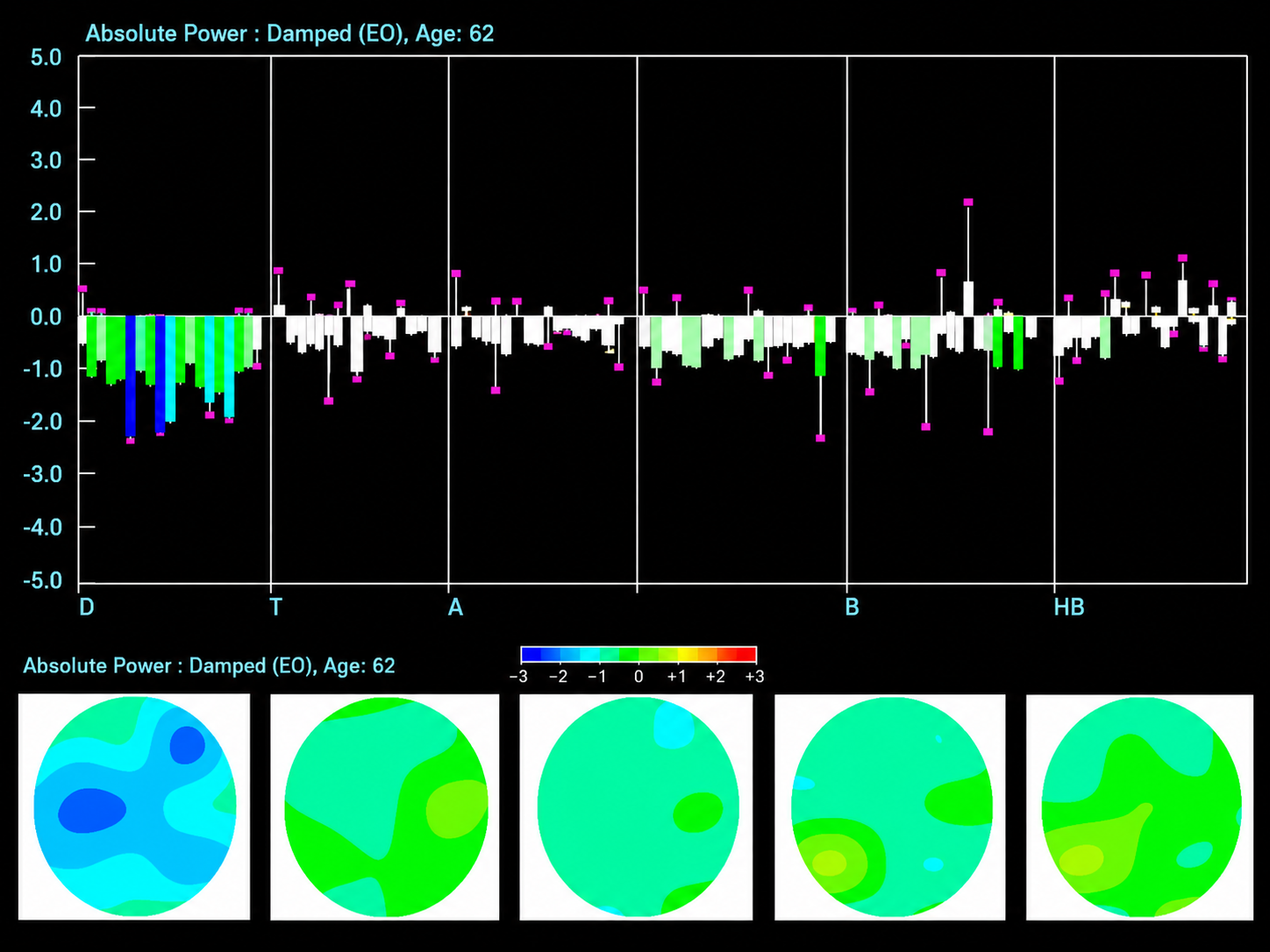
Z-PLUS LZT Live Z-Score Training with Z-Bars and Z-Maps Display.
That count is worth pausing on. Every one of those 76 or 248 values is a separate comparison against a normative distribution, so a handful will fall outside two standard deviations in any recording, including a healthy one. A z-score map is a display of many simultaneous comparisons, not a list of findings.

Tom Collura.
Subsequent advances expanded the method to 19-channel real-time surface z-score training, and then to 19-channel LORETA z-score training, using the mathematical inverse solution of Pascual-Marqui and colleagues (1994) to estimate cortical sources of EEG activity in three dimensions. Robert Thatcher and his team went on to adopt swLORETA, which adds a lead-field weighting to sLORETA to improve robustness under realistic noise and sensitivity to deep sources (Palmero-Soler et al., 2007).
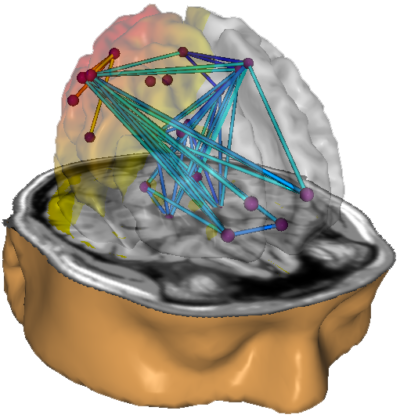
NeuroNavigator swLORETA.
Collura and his colleagues initially used the NeuroGuide database, then shifted to E. Roy John's BrainDX database, and more recently adopted a database known as qEEGPro. The qEEGPro database was developed using client EEG recordings that were cleaned of clinical EEG patterns identified through a client questionnaire (qEEG.pro/database/). This approach is based on assumptions that many qEEG researchers have questioned, and several experts consulted about it expressed skepticism (personal communication, John Anderson, 2019-2021).
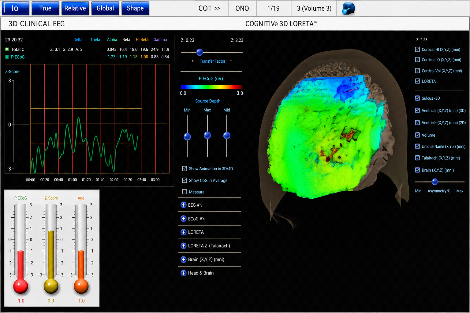
qEEGPro 19-Channel sLORETA Z-Score Training.
The database developer maintains a bibliography of more than 50 z-score neurofeedback publications (https://www.appliedneuroscience.com/PDFs/Z_Score_NFB_Publications.pdf). Read it as a map of activity rather than an efficacy corpus: it mixes peer-reviewed articles with book chapters, newsletter pieces, a dissertation, and single-case reports, and contains no randomized controlled trials. The size of a bibliography is not itself evidence, and a report that leans on one is making a weaker claim than it appears to make.
Clinical Database Development
Alongside the development of the normative database came a parallel tradition. Skilled practitioners who also trained new clinicians began developing what became known as a clinical database, a reference system built from personal experience with often hundreds of clients and from their observations of similarities and differences in EEG findings across clinical populations. They also drew on the published electroencephalography and neurofeedback research to identify correlations with their own experience. This led to several semi-automated approaches to assessment.
Paul Swingle stated in NeuroConnections (Swingle, 2014) that “For Clinicians, the most accurate databases are clearly clinical.” He raised several logical challenges to the normative approach, beginning with the problem of using a group of supposedly "normal" individuals as the reference standard against which a symptomatic client is compared.

Paul Swingle.
Swingle questioned the premise that symptom-free individuals selected for a normative database are truly free of underlying abnormalities. Heritable disorders such as migraine and schizophrenia may have verifiable neurophysiological components that remain unexpressed because triggering factors have not occurred. A database of individuals who pass every screening test might therefore still contain notable EEG findings that become part of the "normal" standard, and Swingle argues that such comparisons are not useful for accurate client assessment.
Others have raised complementary concerns. Johnstone and Gunkelman (2003) pointed out that a symptom-free individual may still show abnormal findings on a clinical EEG assessment performed by a skilled electroencephalographer. They also noted that a database comparison identifies differences from average, not from optimal. The term "normal" is inherently difficult to define, particularly for a measure as variable as the EEG.
Proponents of clinical databases claim exceptional accuracy with clinical populations because these databases were developed from experience with individuals who share similar symptoms, causal factors, symptom progression, and treatment histories. Because of that reported accuracy and their close alignment with client symptomatology, clinical databases are often more descriptive and, some say, more user-friendly.
A practical difference between the two approaches lies in their output. A normative database analysis may produce 200-300 pages of tables, graphs, and topographic brain maps like the ones below. This impressive array of information can be overwhelming and difficult to interpret. Questions arise about which components are important, which relate to the client's symptoms, and which are useful for planning training sessions.
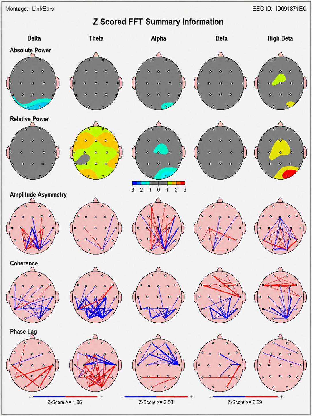
Image from NeuroGuide Normative Database, Applied Neuroscience.
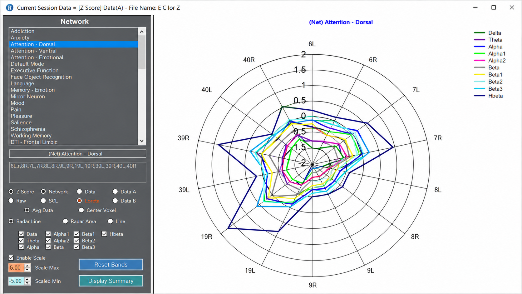
Image from LORETA Progress Report by Phil Jones.
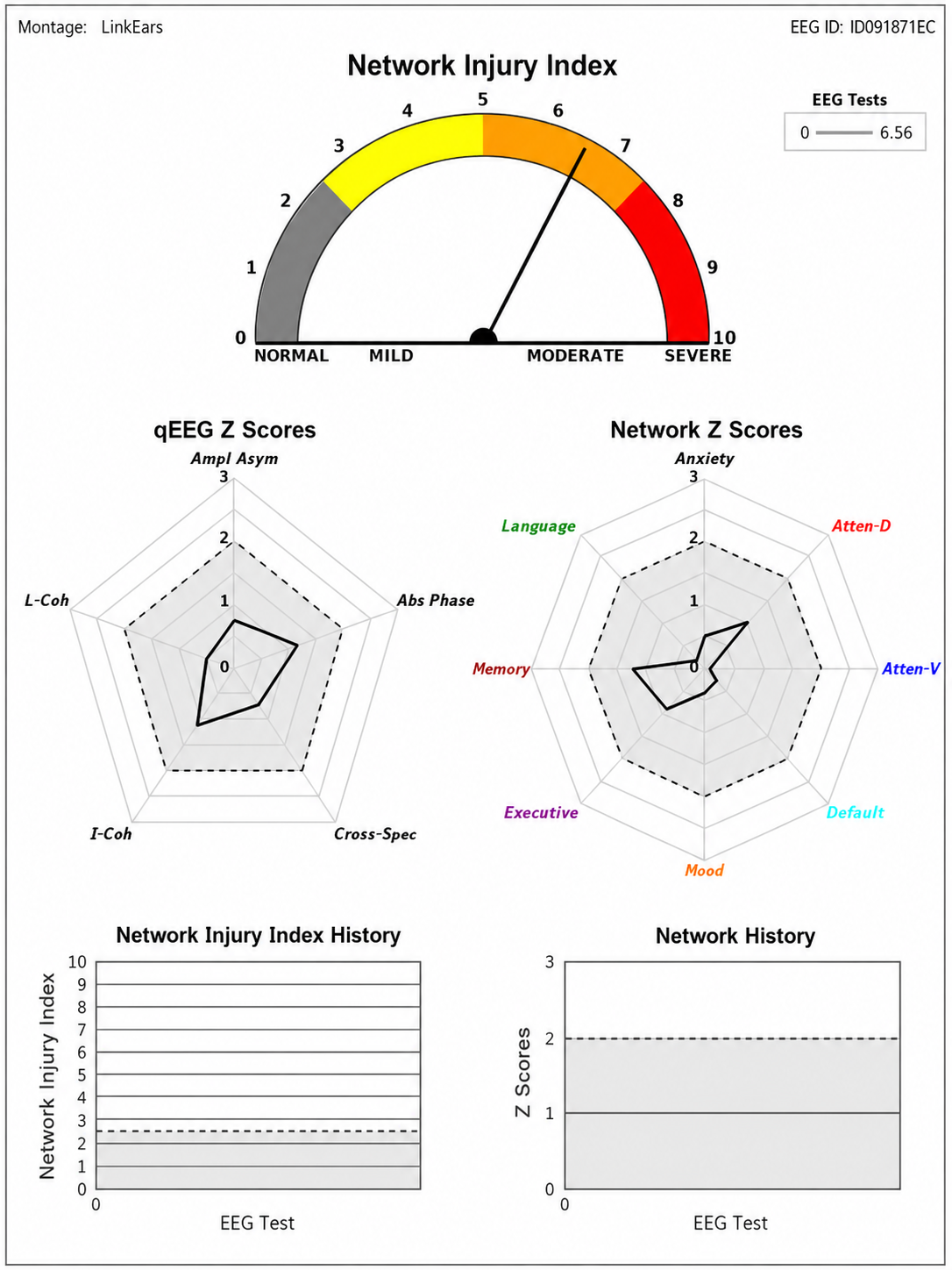
Image from NeuroGuide Normative Database, Applied Neuroscience.
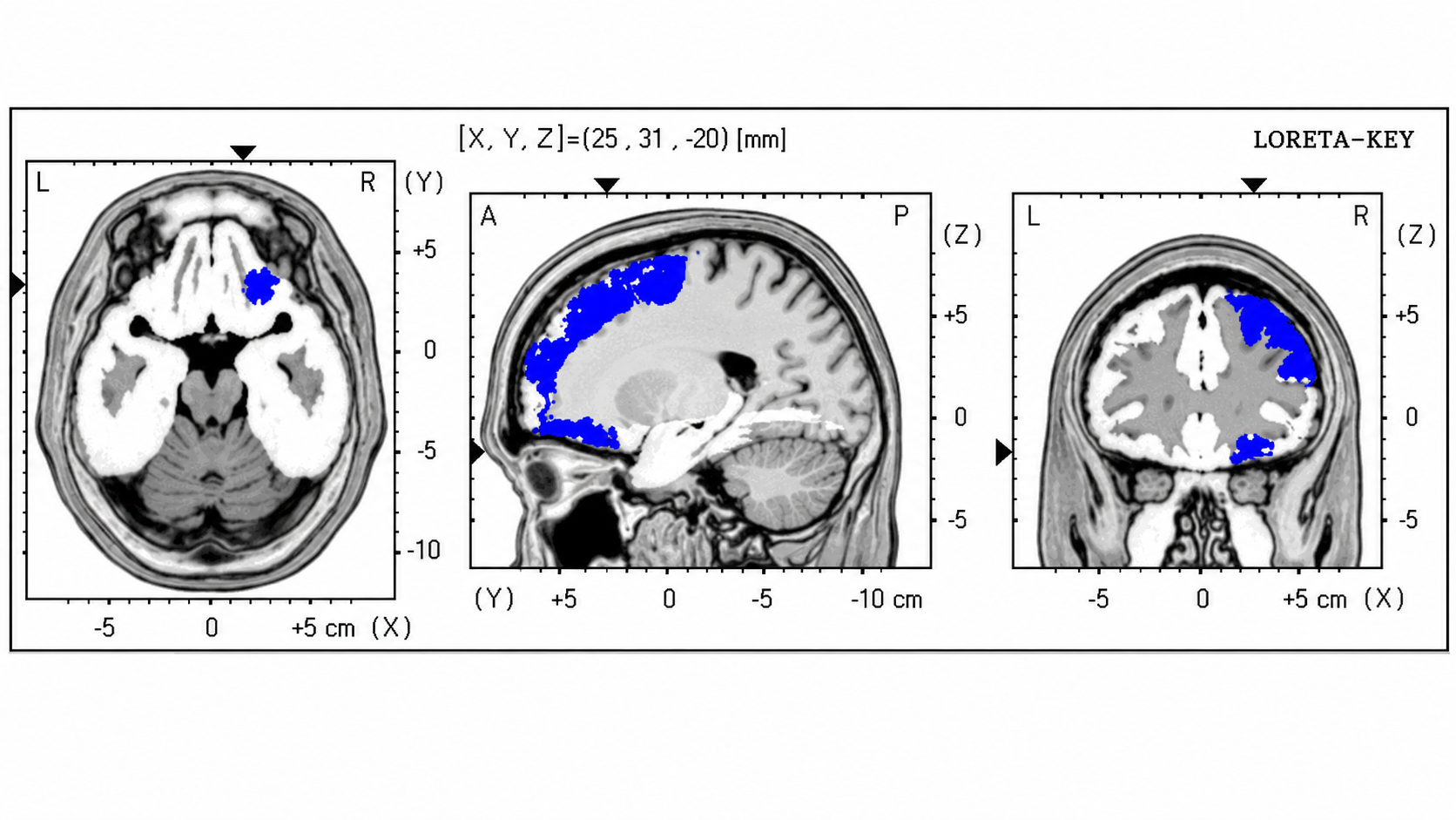
Image from Low Resolution Electromagnetic Tomography (LORETA), Roberto Pascual-Marqui.
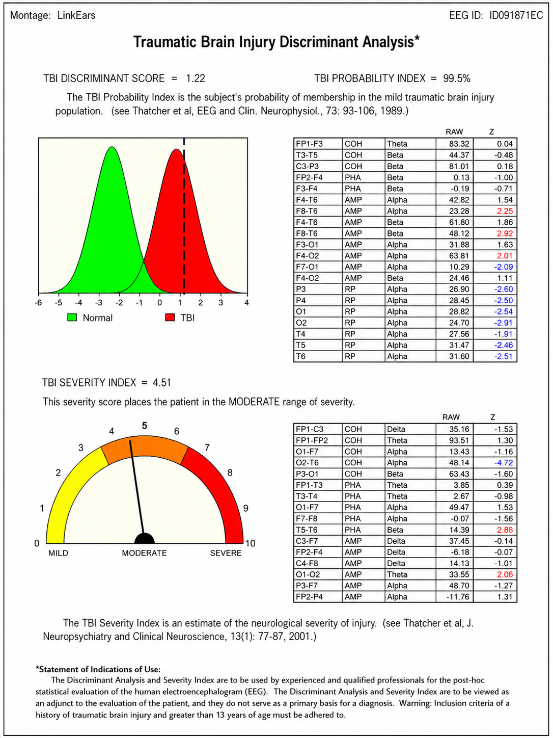
Image from NeuroGuide Normative Database, Applied Neuroscience.
Clinical databases, by contrast, are often more descriptive and closely aligned with client symptomatology. Some provide only graphs and tables, but most also suggest relationships between findings and probable client symptoms. Swingle's Clinical Q, for example, displays differences from expected data and offers "probes," questions about client symptoms or behaviors that may be consistent with specific EEG findings.
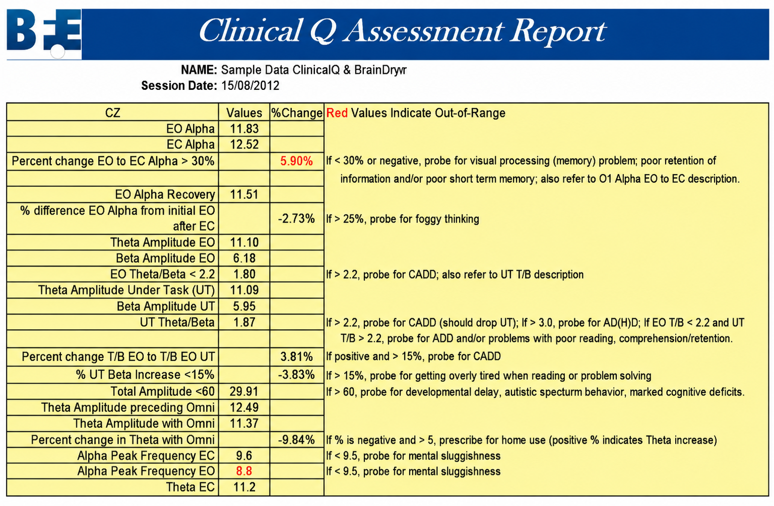
Clinical Q example report.
Peter Van Deusen
One of the earliest clinical databases was created by Peter Van Deusen (Ribas et al., 2016), who initially studied with Joel Lubar. His goal was to identify client symptoms and behavioral issues without relying on diagnostic categories, so that a training approach could be chosen regardless of the specific diagnosis. The culmination of his years of clinical work was an approach known as The Learning Curve (TLC), which organized client symptoms and findings into six broad categories and identified corresponding training approaches.

Peter Van Deusen.
Richard Soutar
Arguably the most comprehensive clinical database system is the New Mind Maps developed by Richard Soutar. This system offers multiple levels of analysis up to 19 channels and produces a detailed report covering most standard metrics. It provides narrative content, protocol recommendations for both standard amplitude training and z-score training, and advice about additional interventions such as audio-visual entrainment (AVE). Because the 19-channel version records all sites simultaneously, it is the one clinical system in this group that can compute phase and coherence.

Richard Soutar.
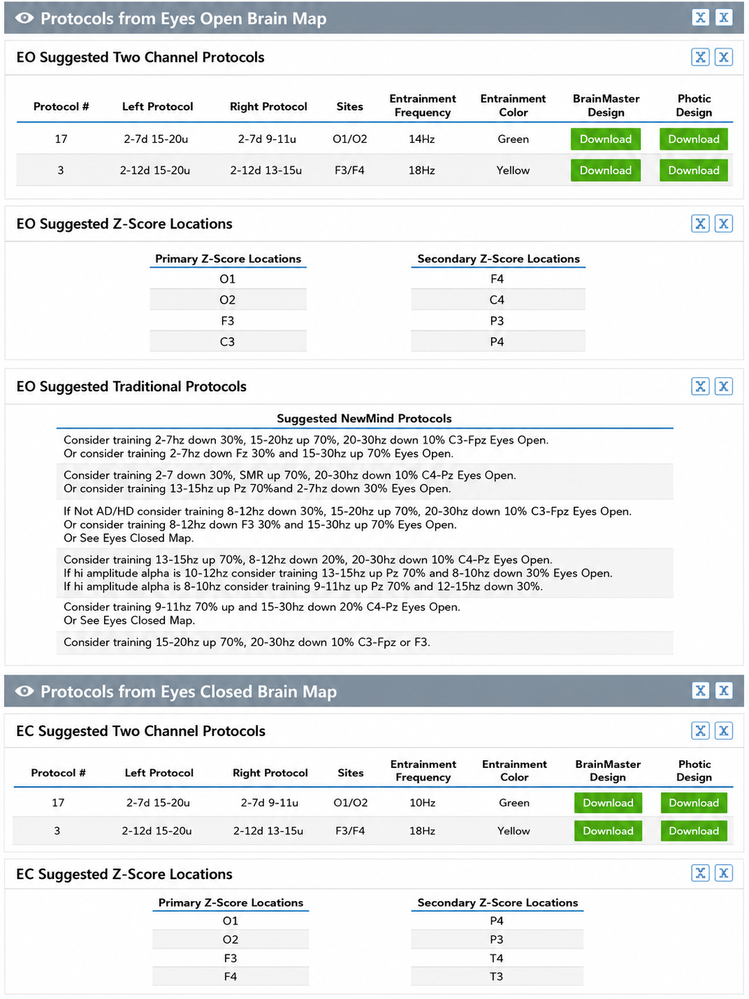
New Mind Maps, Richard Soutar.
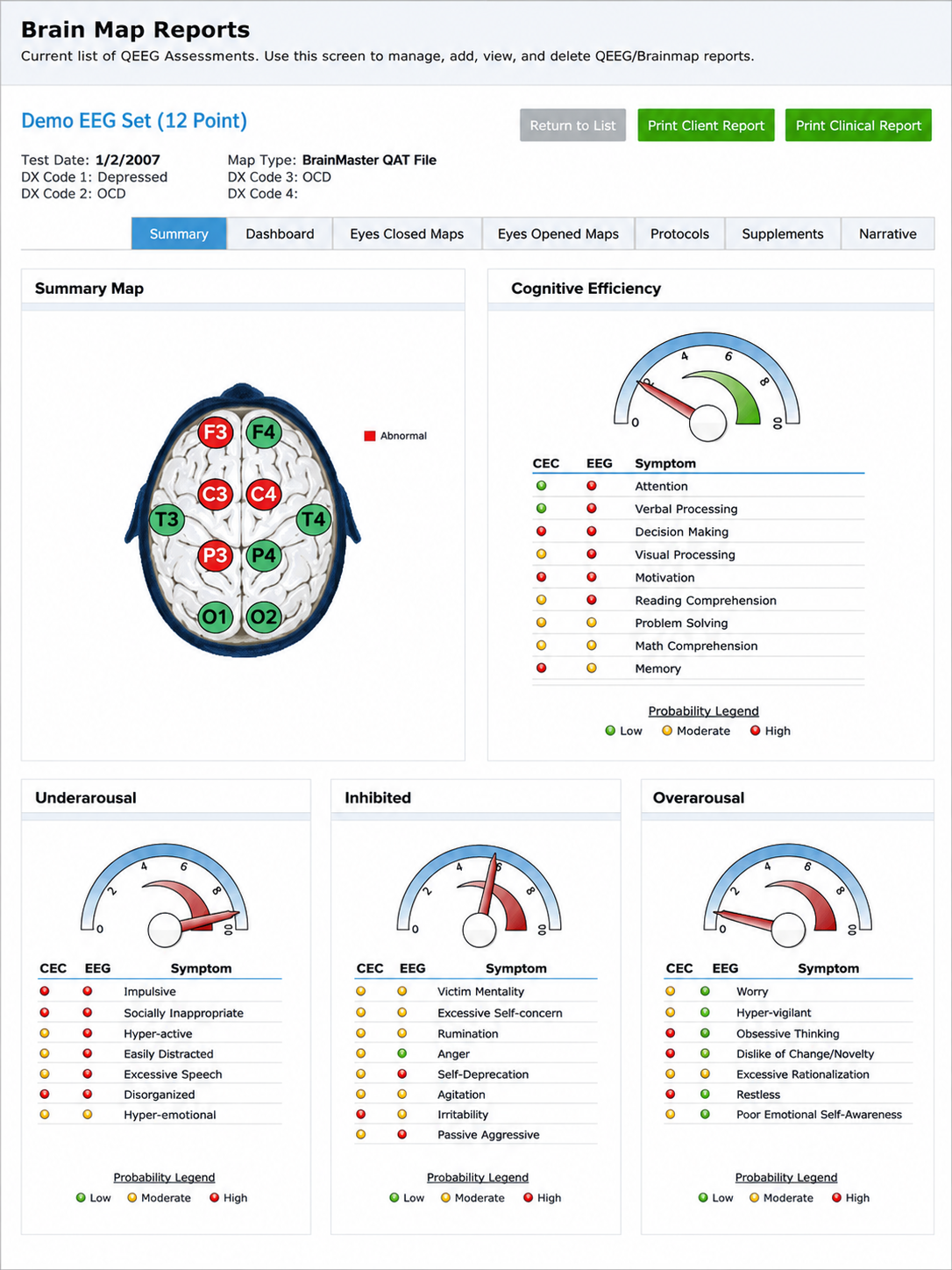
New Mind Maps, Richard Soutar.
John Demos
The Jewel Clinical Database, developed by John Demos, author of Getting Started with EEG Neurofeedback (2nd ed., 2019), provides another clinical database option for ages 7-19 and adults. It produces surface and sLORETA (standardized low resolution electromagnetic tomography) representations including maps, graphs, and training recommendations based on client checklists.
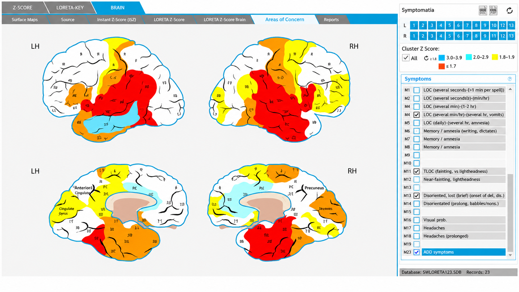
The Jewel Clinical Database, John Demos.

John Demos.
John Anderson
John Anderson developed an assessment specifically for the Nexus/BioTrace system known as the NewQ. Like Swingle's ClinicalQ, which records five sites (Cz, O1, F3, F4, and Fz), it samples a small set of locations sequentially, six locations, two at a time, with four age ranges: 6-11, 12-15, 16-20, and 21+ (adult).

John Anderson.
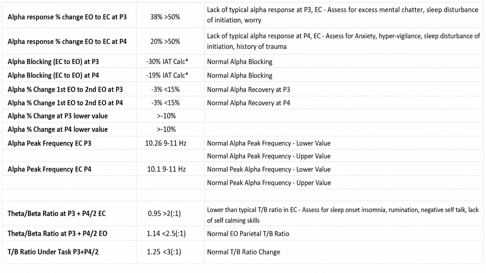
NewQ, John Anderson.
The following disclaimer from the NewQ assessment reflects cautions that apply to every clinical database.
Disclaimer: This assessment tool is based upon a general understanding of the EEG literature plus the author's clinical experience. It should not be viewed as a statistically validated or rigorously referenced instrument and constitutes a set of clinical observations. It is not a diagnostic instrument, and results must be evaluated based on the client's presenting concerns. The clinical judgment of the practitioner must remain primary in any assessment process.
The clinical database approach has genuine value. It provides practitioners with assessment perspectives grounded in the author’s knowledge and clinical experience, offering a helpful shortcut for beginning and experienced clinicians alike.
However, because sensor locations are often recorded sequentially (except for Soutar’s 19-channel New Mind Maps), these assessments cannot calculate important metrics such as phase and coherence for locations not recorded simultaneously. That limitation matters for the montage comparison later in this unit, since every connectivity measure discussed there requires simultaneous recording. Additionally, each designer’s perspective is inherently subjective and, while reflecting real knowledge and experience, may also carry unconscious biases and assumptions not rigorously grounded in published research.
Ideally, the field will eventually integrate the normative database approach with clinical assessment to create a truly accurate and effective expert system for developing evidence-based training protocols.
Topographic mapping turns preprocessed, spectrally analyzed EEG into a spatial picture by interpolating values between electrodes and color coding the result. Its benefits are enhanced visualization, localization of brain function, and improved diagnostic accuracy. Two traditions of database development grew up alongside it. The normative approach, developed by Thatcher and Collura, compares a client against age-matched controls and expresses differences as z-scores. A two-channel comparison produces roughly 76 of those values and a four-channel comparison up to 248, so some will fall outside two standard deviations in any recording and a map is a display of many simultaneous comparisons rather than a list of findings. The clinical approach, developed by Swingle, Van Deusen, Soutar, Demos, and Anderson, compares a client against a practitioner's accumulated experience with similar presentations and maps findings onto probable symptoms.
Check Your Understanding
- What preprocessing steps must precede spectral analysis, and why does each matter for the resulting map?
- How does interpolation between electrodes create a continuous map, and what does that imply about the areas between sensors?
- Trace live z-score training from the early two- and four-channel systems to swLORETA. What did each step add?
- Roughly how many z-scores does a two-channel comparison produce, and why does that number matter when you read a z-score map?
- What is Swingle's objection to using symptom-free individuals as a normative reference standard?
- What limitation do sequentially recorded clinical assessments share, and which metrics does it put out of reach?
A Guide to Interpreting qEEG Topographic Maps
Reading topographic maps of the EEG may seem straightforward and relatively simple. Z-score maps highlight areas that deviate from typical values compared to normative databases adjusted for age and sometimes gender and handedness. When an area on the map shows excessive activity in a particular EEG frequency, targeted sensor placement and effective client training can help normalize these levels. Conversely, reduced activity in an area may result in efforts to enhance it.
However, the reality is more complex. EEG recordings often exhibit significant artifacts from multiple sources, such as environmental interference (e.g., 50- or 60-Hz electrical noise) and physiological factors like eye blinks, movements, heartbeats, and muscle contractions. We must clean EEG data to ensure its integrity. This requires distinguishing between genuine EEG activity and transient phenomena such as drowsiness, sleep, or normal variants that do not signify pathology. While important for an accurate EEG report, these EEG features should not factor into statistical analyses.
Creating topographic EEG maps should be considered one of the last stages of a clinical assessment, not its primary focus.
Therefore, adhering to a careful progression from data collection to comprehensive analysis is essential instead of relying on automated artifact rejection algorithms and immediately generating maps.
Focusing neurofeedback training on areas associated with problematic symptoms is important for effective intervention. Simply targeting any abnormality detected in the EEG may not address the underlying issues and could lead to unintended consequences.
Atypical EEG findings can arise from various factors, including exceptional skills, compensatory changes due to illness or injury, developmental differences, or unique characteristics that do not necessarily indicate pathology. Therefore, careful clinical assessment and interpretation are necessary to determine whether observed deviations require correction.
By focusing on symptom-based training associated with understanding the clinical picture, clinicians can ensure that neurofeedback protocols address specific concerns and optimize outcomes for individuals undergoing training.
The following is an example of an EEG recording of a 76-year-old male with complaints of "brain fog," memory problems, lack of energy, slow cognitive processing, and difficulty sleeping.
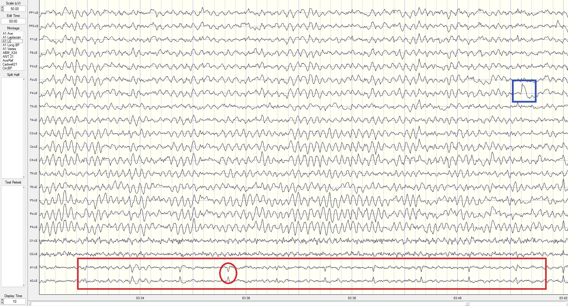
Eyes-Closed Linked Ears (ECLE) Montage
This is a 50-uV scale, 10-sec display. Note the persistent ECG artifact in multiple channels, most clearly seen in reference channels (red outline at the bottom). The peak alpha frequency is approximately 8 Hz, the amplitude is 12-25 uV at the parietal sensors, and there is a small electrode pop in the F4 sensor (blue outline in this and subsequent montages).
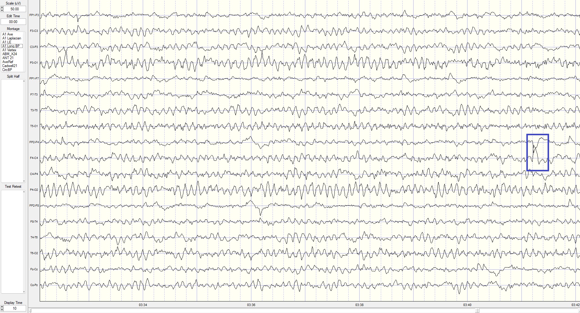
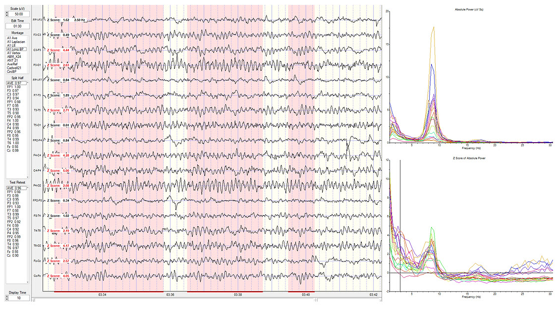
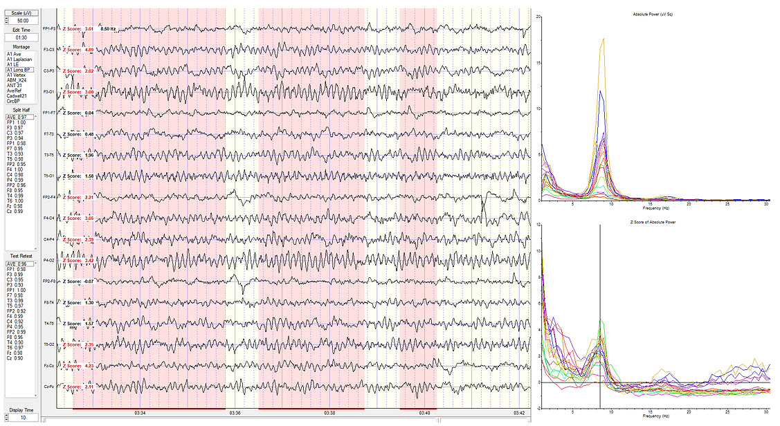
Eyes-Closed Longitudinal Bipolar (ECLBP) Montage
This is a 50-uV scale, 10-second display. The alpha frequency is 8 Hz, and the amplitude is 10-30 uV in parietal-occipital derivations. Note that the rhythmic activity (frontal alpha) seen in the linked ears montage is not present in prefrontal-frontal derivations in this bipolar montage, indicating it was the result of reference contamination in the previous montage.
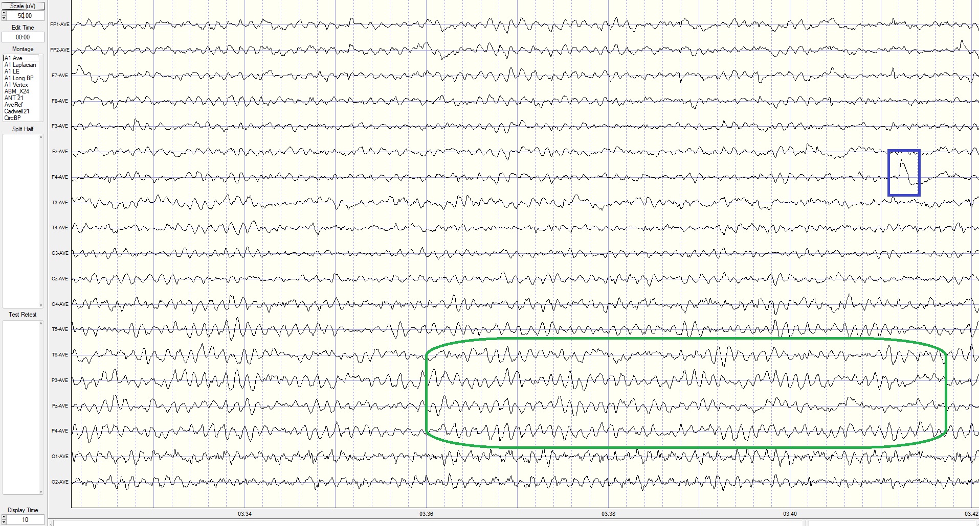
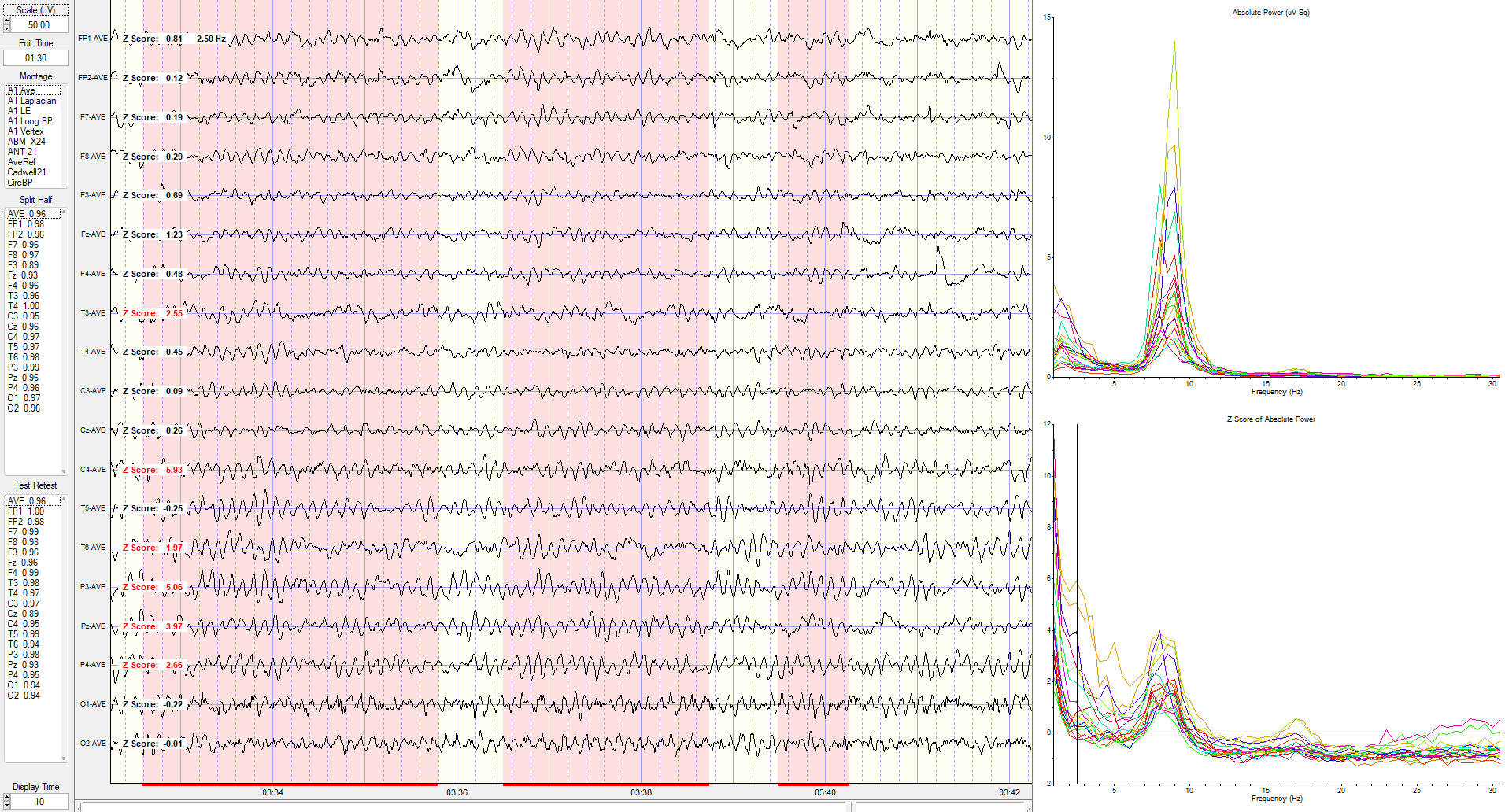
Eyes-Closed Average Reference (ECAVE) Montage
This is a 50-uV scale, 10-second display. The alpha frequency is 8-9 Hz, and the amplitude is 5-15 uV at the occipital and 10-18 uV at the parietal sensors. Note the delta activity at the parietal sensors (green outline) and EMG artifact at the occipital sensors.
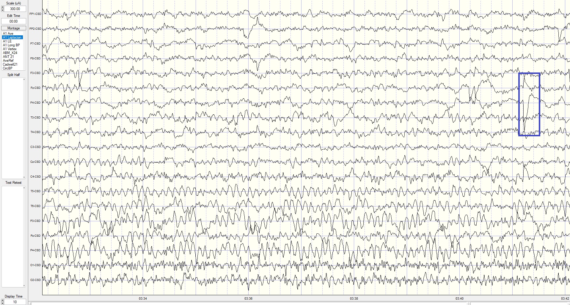
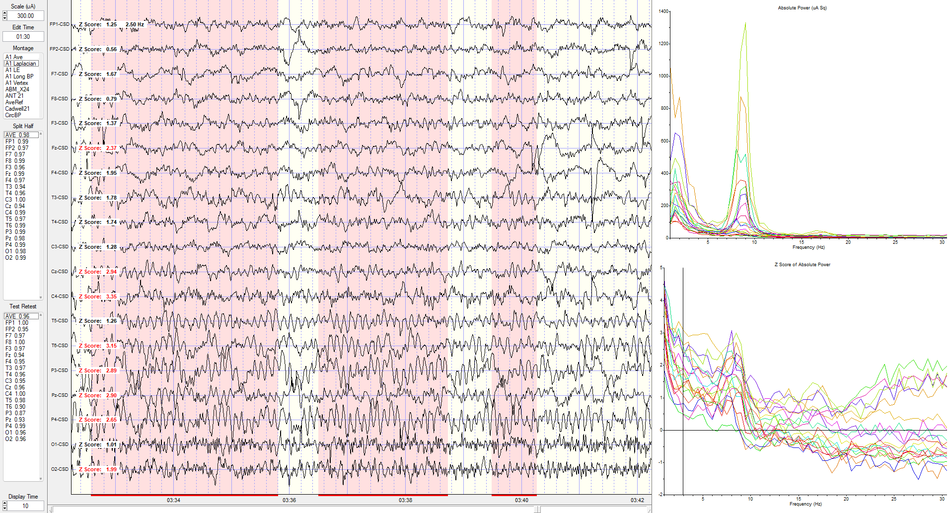
Eyes-Closed Laplacian (ECLP) Montage
This is a 400-microampere (uA) scale, 10-second display. The alpha frequency is 8-9 Hz, with the highest current density in parietal sensors. EMG artifact continues in occipital sensors, and delta is more pronounced in the parietal area. Electrode pop in F4 sensor. The lack of prefrontal and frontal alpha activity suggests reference contamination in the linked ears montage above.
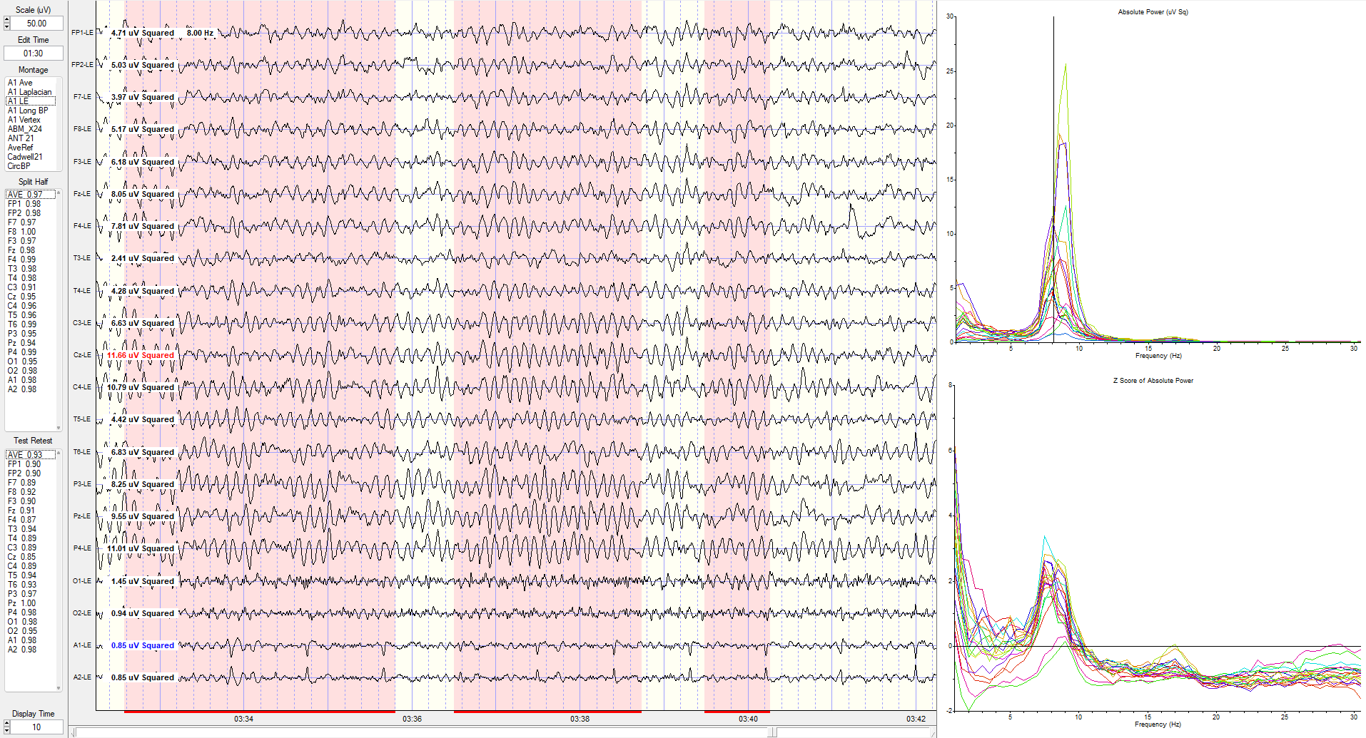
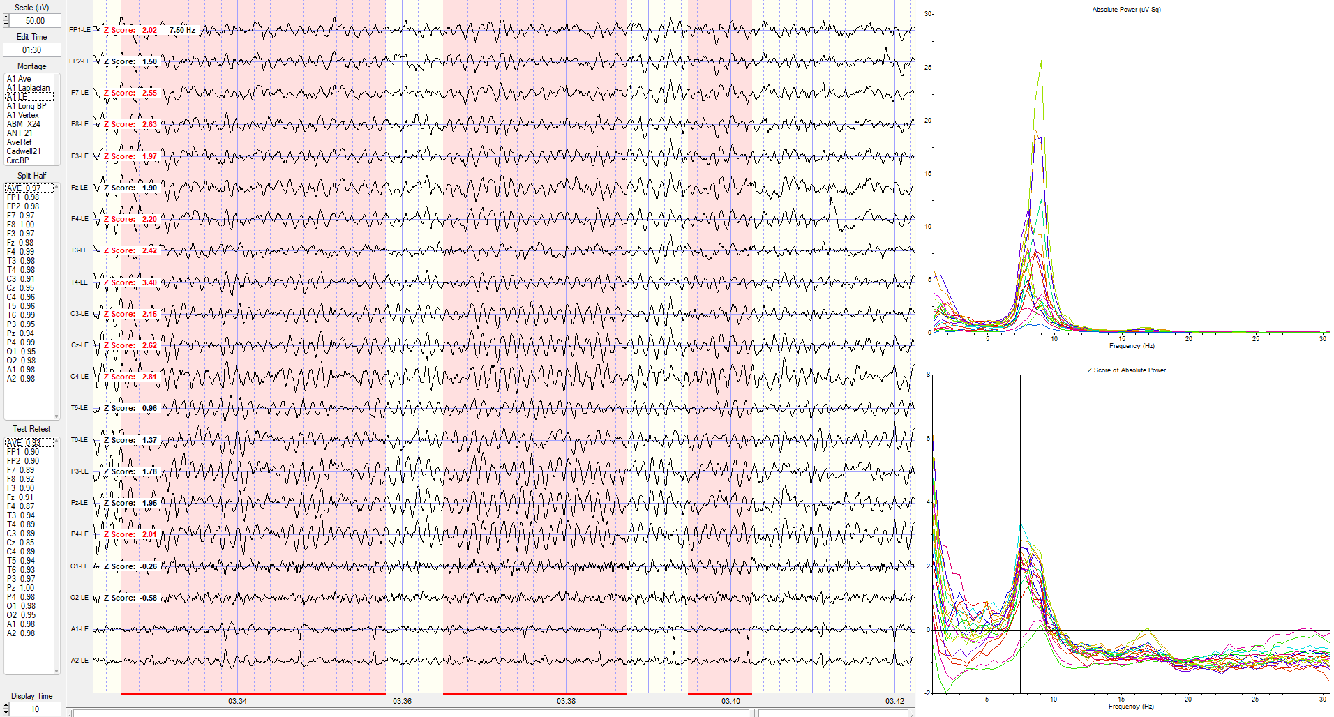
Eyes-Closed Linked Ears (ECLE) Montage
A linked ears montage in NeuroGuide with FFT absolute power spectral display at the top right with a line indicating the highest amplitude at 9 Hz is at the P4 electrode.
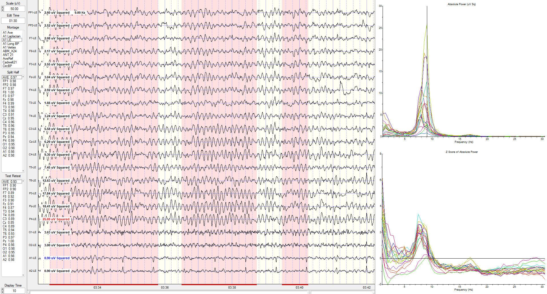
The same image showing the maximum power at 8 Hz is at the C4 electrode.
The same linked ears montage image shows the peak activity at 7.5 Hz, which is generally 1-3 SD greater than typical values at multiple locations (see z-score indicators on the left side of tracings next to electrode location labels).
Eyes-Closed Longitudinal Bipolar (ECLBP) Montage
This spectral display shows a longitudinal bipolar montage indicating the maximum z-scores at 2.5 Hz.
Eyes-closed longitudinal bipolar montage showing standard deviations at 8.5 Hz.
Eyes-Closed Average Reference (ECAVE) Montage
Average reference montage showing deviations at 2.5 Hz.
Eyes-Closed Laplacian (ECLP) Montage
Laplacian montage showing current source density (CSD) z-scores at 3 Hz.
Eyes-Closed Linked Ears (ECLE) Montage
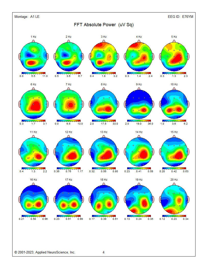
These absolute power topographic maps represent 1 minute and 30 seconds of a recording from an eyes-closed linked ears montage. Each small head map represents a virtual view of the top of the head with the nose at the top. The absolute power (microvolts squared) values correspond to the colored scale below each map.
Red represents the greatest value, and blue is the lowest value for each 1 Hz frequency bin. The P4 electrode shows a power value of 36 in the 9 Hz frequency bin. Each bin has its own scale.
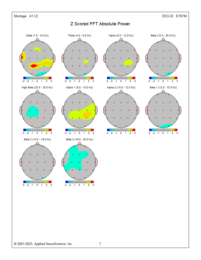
Z-Score Absolute Power
1-Hz frequency bin maps showing maximum to minimum deviations compared to the NeuroGuide normative database for a linked ears montage. The scale is from -3 (blue) to +3 (red) standard deviations (SD). The excess activity at 1 Hz is likely due to the ECG artifact noted earlier. The heart beats at about 1 beat per second, which equals 1 Hz. Excess activity is seen at 7-9 Hz.
Frequency band maps (like delta, theta, alpha, and beta) show the entire frequency band and lack the resolution of the individual 1-Hz frequency bin maps. The delta map generally shows excess delta activity, which misidentifies the ECG artifact that was seen at 1 Hz in the frequency bin maps and the visual inspection of the EEG.
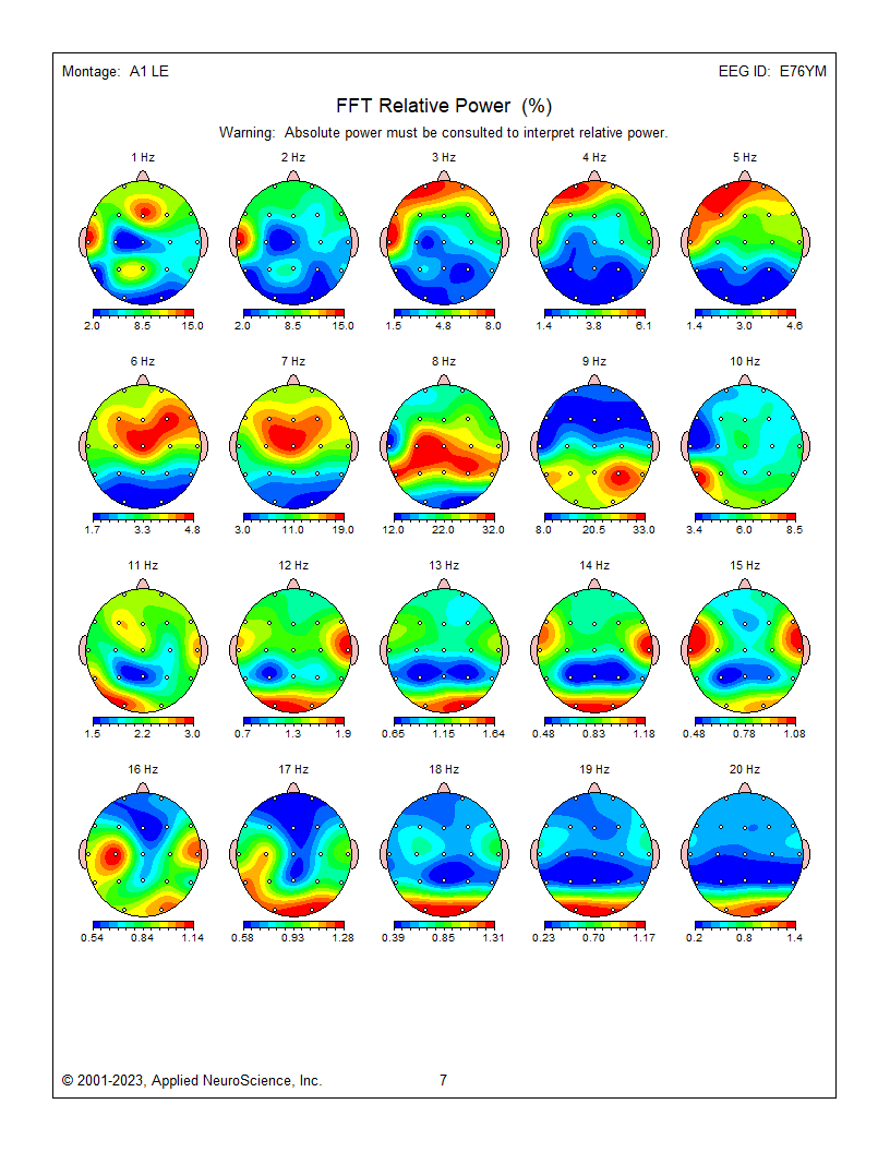
These are relative power topographic maps representing 1 minute and 30 seconds of data from an eyes-closed linked ears montage. They show relative power values (percentages) that compare the value in each 1 Hz bin to the broadband EEG (0.5 to 30 Hz). This information is displayed as a colored scale below each map, with red representing the highest percentage and blue representing the lowest percentage for each 1-Hz frequency bin. Note that 9 Hz contains 33 percent of the total EEG power at the P4 electrode location. Each head map has its own scale.
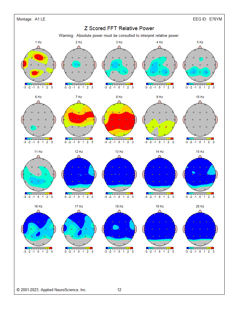
These are z-score relative power 1-Hz frequency bin maps showing maximum to minimum deviations compared to the NeuroGuide normative database using a linked ears montage. The scale is from -3 (blue) to +3 (red) standard deviations (SD). Note that this page represents relative power, showing the relative value of each 1 Hz bin compared to the EEG as a whole. This can result in areas showing incorrect abnormal z-score values at some frequencies because other frequencies are abnormal in the opposite direction. For example, frontal, central, and parietal activity at 8 Hz is excessive in the image below, causing apparent deficient activity in the same areas at multiple frequencies because 8 Hz takes up too much of the percentage "pie."
The previous examples show the progression of EEG analysis from viewing the recorded EEG through spectral analysis to topographic maps representing absolute and relative power and z-score maps showing deviations from expected values when client results are compared to a normative database.
The raw tracings and the spectral displays show examples from multiple montages (sensor comparisons) and help to highlight that what is seen depends heavily on which comparisons are used. So far the topographic map examples have all used the linked ears montage and showed only one perspective on the EEG results. Now we will look at the same data presented as topographic maps using different montages.
Eyes-Closed - 3 Montages
Eyes-closed average montage absolute power topographic map for 1-20 Hz, eyes-closed linked ears absolute power topographic map for 1-20 Hz, and eyes-closed Laplacian absolute power topographic map for 1-20 Hz.
.png)
.png)
.png)
Eyes-closed average z-score absolute power topographic map for 1-20 Hz, eyes-closed linked ears z-score absolute power topographic map for 1-20 Hz, and eyes-closed Laplacian montage z-score absolute power topographic map for 1-20 Hz. Notice the differences between the average, Laplacian, and linked ears reference maps. Which one should we follow when completing our assessment?
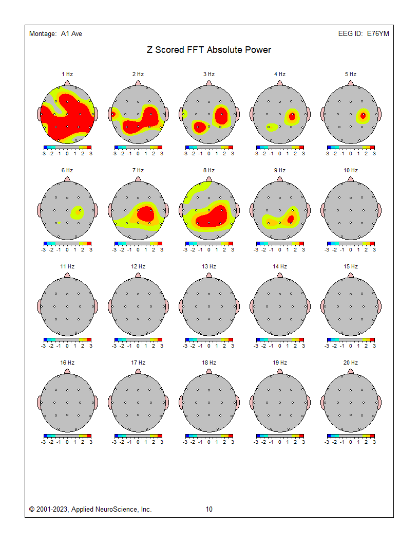
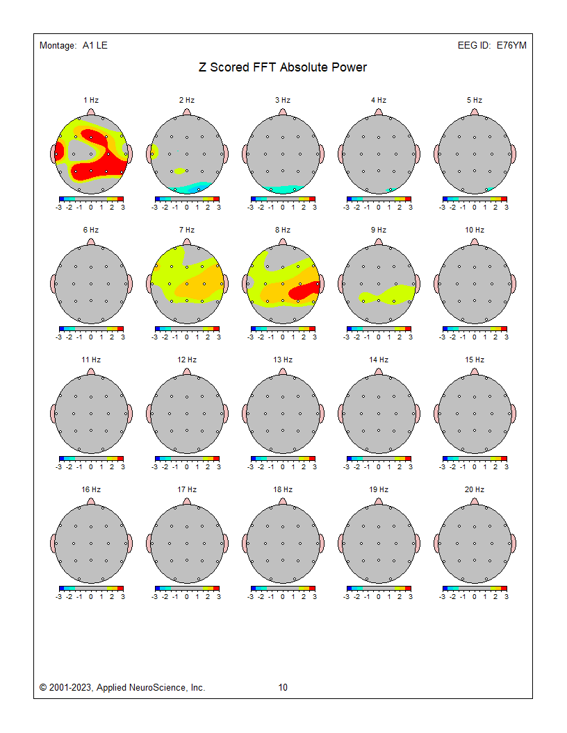
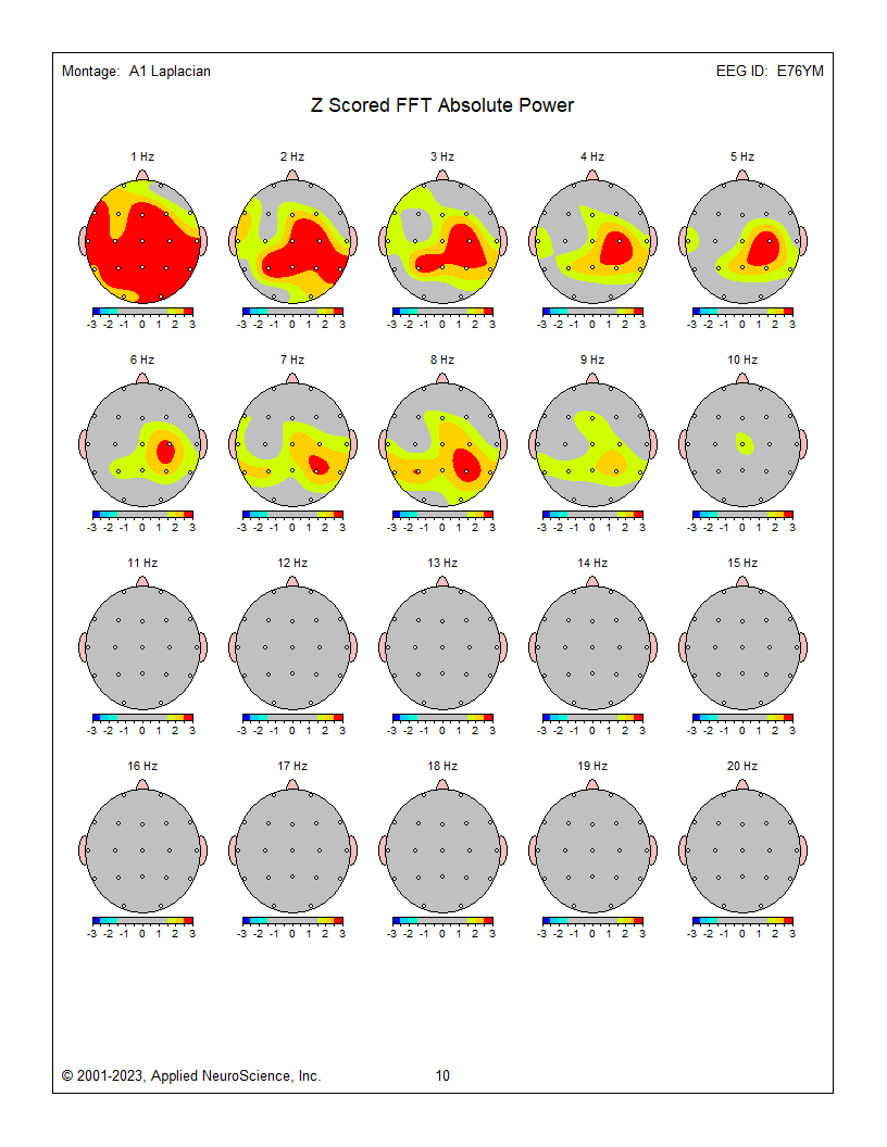
The average reference and Laplacian montages show fairly similar results and correspond to some of the other indicators and may generally represent the client’s presenting issues of brain fog, memory issues, and slow cognitive processing.
Several posts and Neurofeedback Tutor have addressed the issue of montage selection. Nunez and Srinivasan's (2006) Electrical Fields of the Brain (2nd ed.) is an excellent resource for more in-depth information.
For this example, we are confronted with significant differences between the linked ears results and average reference and Laplacian montage results, when there is excess activity in the 2-6 Hz range of delta and theta.
The Laplacian montage uses an average of the current flow from electrodes immediately surrounding the electrode of interest as a localized average reference using current rather than voltage as its metric. This has been described as more accurate in identifying local activity while minimizing general effects such as those from medication, drowsiness, and others. This can help highlight local abnormalities, which can be lost or masked by other montages.
The average reference montage uses an average of all scalp electrodes to serve as the reference for each electrode, thus eliminating the ear or mastoid reference. This helps remove contributions from these reference electrodes, common to all electrode pairings when using the linked ears or linked mastoid reference montage.
Each of these montage choices has benefits and limitations. The benefits have been mentioned above, but what are the limitations? The average reference montage, like all montages, is subject to the differential amplifier's common mode rejection phenomenon.
Sources (electrical activity such as EEG, ECG, EMG, EOG, EMF) that are the same in frequency and, to a lesser extent, in amplitude are rejected, while sources that are different are retained. If multiple sources (electrode locations) of delta activity contribute to the average, and this average is then compared to a location that does not show delta activity, then there is a difference between the signals. That difference is retained and displayed in the topographic maps and, of course, in the EEG tracings, resulting in apparently abnormal delta activity where it does not exist.
The same is true of the linked ears/mastoid reference and, to a lesser extent, of the Laplacian montage.
Therefore, we look for agreement among multiple montages, being particularly attentive to the various bipolar montages that allow revealing comparisons when viewing the EEG tracings.
In the present example, though earlier we mentioned that the delta activity was confined to the 1 Hz effect from the ECG (heartbeat) artifact, we can see from the Laplacian and average montages that there is substantial agreement on a broader frequency distribution of delta/theta activity that exceeds statistical significance. Thus, the recommendation is to begin training by focusing on these excesses.
The same recording produces different maps depending on the montage you choose, so montage selection is an interpretive act rather than a neutral display setting. Frontal alpha that appears in a linked ears montage but vanishes in a bipolar montage was reference contamination, not brain activity. Common mode rejection means that shared activity is rejected while differing activity is retained, so an average or linked ears reference can manufacture apparent abnormality where none exists. Build maps near the end of an assessment, after artifact has been addressed by hand, and train the findings that connect to the client's presenting symptoms rather than every deviation the software flags.
Check Your Understanding
- Why should topographic mapping come near the end of a clinical assessment rather than at its start?
- In the worked example, what told you that the frontal alpha in the linked ears montage was reference contamination?
- How can common mode rejection produce apparently abnormal delta activity where none exists?
- Name three reasons an atypical EEG finding might not indicate pathology.
- Why is targeting every abnormality the software detects a poor training strategy?
Assignment
Now that you have completed this unit, explain the rationale for z-score training using a normative database. Then argue the opposing case: what would a clinical-database advocate say in reply, and how would you decide between the two approaches for a particular client?
Glossary
bins: frequency ranges, which may be as narrow as 1 Hz, into which the EEG power spectrum is divided.
clinical database: a reference set built from a clinician's accumulated experience with clinical populations that maps EEG findings onto probable client symptoms and suggests training approaches.
EEG power: the squared amplitude of EEG activity quantified over time or frequency, expressed as µV² for band power or µV²/Hz for power spectral density.
eyes-closed average reference (ECAVE) montage: an eyes-closed EEG recording referenced to the mean of all scalp channels, which is subtracted from each channel to suppress activity common to all sites.
eyes-closed Laplacian (ECLP) montage: an eyes-closed EEG recording transformed by the surface Laplacian, which emphasizes activity local to each electrode and reduces the influence of distant sources, sharpening spatial resolution.
eyes-closed linked ears (ECLE) montage: an eyes-closed EEG recording referenced to earlobe electrodes that are electrically joined, giving a stable reference shared by both hemispheres.
eyes-closed longitudinal bipolar (ECLBP) montage: an eyes-closed EEG recording displayed as anterior-to-posterior chains of electrode pairs, each channel showing the voltage difference between two neighboring sites.
Live Z-Score Training (LZT): a neurofeedback approach that provides real-time information about how closely a client's EEG matches an age-matched normative database, with differences displayed in standard deviations.
low-resolution electromagnetic tomography (LORETA): the inverse solution of Pascual-Marqui and colleagues (1994) that estimates three-dimensional cortical sources of scalp-recorded EEG at low spatial resolution.
montage: the specified arrangement of electrode derivations or channel pairings used to display a physiological recording.
normative database: a reference set of EEG measures collected from healthy subjects across age ranges, against which an individual client's values are compared as z-scores.
quantitative electroencephalography (qEEG): the statistical analysis of digitized EEG, which produces objective and quantifiable measures of brain function such as absolute and relative power, ratios, asymmetry, and connectivity.
sLORETA: standardized low-resolution brain electromagnetic tomography, a version of LORETA that standardizes the current density estimate to achieve zero localization error under ideal conditions (Pascual-Marqui, 2002).
swLORETA: a version of sLORETA that adds a singular-value-decomposition-based lead-field weighting, improving localization under realistic noise and for deep sources (Palmero-Soler et al., 2007).
z-score absolute power: the number of standard deviations by which a client's absolute power in a given frequency band and site departs from the age-matched normative database mean.
Test Yourself on ClassMarker
Click the button below to take a 10-question exam over this entire unit. There is no password.
Review Flash Cards on Quizlet
Click the button below to review our chapter flash cards.
References
Demos, J. N. (2019). Getting started with EEG neurofeedback (2nd ed.). W. W. Norton.
Johnstone, J., & Gunkelman, J. (2003). Use of databases in QEEG evaluation. Journal of Neurotherapy, 7(3-4), 31–52. https://doi.org/10.1300/J184v07n03_02
Nunez, P. L., & Srinivasan, R. (2006). Electric fields of the brain: The neurophysics of EEG (2nd ed.). Oxford University Press. https://doi.org/10.1093/acprof:oso/9780195050387.001.0001
Palmero-Soler, E., Dolan, K., Hadamschek, V., & Tass, P. A. (2007). swLORETA: A novel approach to robust source localization and synchronization tomography. Physics in Medicine and Biology, 52(7), 1783–1800. https://doi.org/10.1088/0031-9155/52/7/002
Pascual-Marqui, R. D. (2002). Standardized low-resolution brain electromagnetic tomography (sLORETA): Technical details. Methods and Findings in Experimental and Clinical Pharmacology, 24(Suppl. D), 5–12.
Pascual-Marqui, R. D., Michel, C. M., & Lehmann, D. (1994). Low resolution electromagnetic tomography: A new method for localizing electrical activity in the brain. International Journal of Psychophysiology, 18(1), 49–65. https://doi.org/10.1016/0167-8760(84)90014-X
Ribas, V. R., Ribas, R., & Martins, H. (2016). The learning curve in neurofeedback of Peter Van Deusen: A review article. Dementia & Neuropsychologia, 10(2), 98–103. https://doi.org/10.1590/S1980-5764-2016DN1002005
Swingle, P. G. (2014, Spring). Clinical versus normative databases: Case studies of Clinical Q assessments. NeuroConnections.
Thatcher, R. W., Lubar, J. F., & Koberda, J. L. (2019). Z-Score EEG biofeedback: Past, present, and future. Biofeedback, 47(4), 89–103. https://doi.org/10.5298/1081-5937-47.4.04
Return to Top